QTL analysis for Crichton
Hao He
Last updated: 2022-12-24
Checks: 7 0
Knit directory: QTL_analysis_for_Crichton/
This reproducible R Markdown analysis was created with workflowr (version 1.6.2). The Checks tab describes the reproducibility checks that were applied when the results were created. The Past versions tab lists the development history.
Great! Since the R Markdown file has been committed to the Git repository, you know the exact version of the code that produced these results.
Great job! The global environment was empty. Objects defined in the global environment can affect the analysis in your R Markdown file in unknown ways. For reproduciblity it’s best to always run the code in an empty environment.
The command set.seed(20221224) was run prior to running the code in the R Markdown file. Setting a seed ensures that any results that rely on randomness, e.g. subsampling or permutations, are reproducible.
Great job! Recording the operating system, R version, and package versions is critical for reproducibility.
Nice! There were no cached chunks for this analysis, so you can be confident that you successfully produced the results during this run.
Great job! Using relative paths to the files within your workflowr project makes it easier to run your code on other machines.
Great! You are using Git for version control. Tracking code development and connecting the code version to the results is critical for reproducibility.
The results in this page were generated with repository version 92ecd1d. See the Past versions tab to see a history of the changes made to the R Markdown and HTML files.
Note that you need to be careful to ensure that all relevant files for the analysis have been committed to Git prior to generating the results (you can use wflow_publish or wflow_git_commit). workflowr only checks the R Markdown file, but you know if there are other scripts or data files that it depends on. Below is the status of the Git repository when the results were generated:
Ignored files:
    Ignored:    .Rproj.user/

Untracked files:
    Untracked:  analysis/workflow_proc.R
    Untracked:  data/Report-12-27-2019.csv
    Untracked:  data/WT144_GBS_Rqtl_input.csv
Note that any generated files, e.g. HTML, png, CSS, etc., are not included in this status report because it is ok for generated content to have uncommitted changes.
These are the previous versions of the repository in which changes were made to the R Markdown (analysis/QTL_analysis_for_Crichton.Rmd) and HTML (docs/QTL_analysis_for_Crichton.html) files. If you’ve configured a remote Git repository (see ?wflow_git_remote), click on the hyperlinks in the table below to view the files as they were in that past version.
| File | Version | Author | Date | Message |
|---|---|---|---|---|
| Rmd | 92ecd1d | xhyuo | 2022-12-24 | First build |
Library
library(ggplot2)
library(gridExtra)
library(qtl)
library(qtlcharts)
library(tidyverse)
library(lme4)
library(lmerTest)
library(qtl2)
library(cowplot)
Quote from “https://jacksonlaboratory.atlassian.net/wiki/spaces/KL/pages/29794140/WT144+QTL+results”
“The GBS mapping can be found under: /projects/kumar-lab/peera/WT144_GBS_analysis/scripts Overall 225 markers passed genotyping QC, all samples matched the sex. The R code used here can be found here: https://bitbucket.jax.org/users/peera/repos/wt144_scripts/browse I took the input file and ran lm with the formula: TotalDist ~ gender + animal_name * TestAge and extracted the coefficients for the animal alone and the interaction with age. For some reason the distribution of the animal coefficients alone is bi-modal.”
The data was prepared using a nextflow pipeline which is deposited in another repo. The data is ready as a R/qtl input file, it’s being read and scanone/scantwo are run on the data.
Load qtl data and plot summary
WT144 <- read.cross(format = "csv", file = "data/WT144_GBS_Rqtl_input.csv", genotypes = c("A", "H", "B")) --Read the following data:
309 individuals
225 markers
11 phenotypes
--Cross type: f2 chror <- as.character(1:19)
WT144$geno <- WT144$geno[chror]
summary(WT144) F2 intercross
No. individuals: 309
No. phenotypes: 11
Percent phenotyped: 100 100 100 99.7 100 100 99.7 90.9 100 99.7 90.9
No. chromosomes: 19
Autosomes: 1 2 3 4 5 6 7 8 9 10 11 12 13 14 15 16 17 18 19
Total markers: 225
No. markers: 18 23 17 15 46 1 19 4 8 3 5 18 11 10 2 4 7 2 12
Percent genotyped: 85
Genotypes (%): AA:40.6 AB:46.9 BB:12.5 not BB:0.0 not AA:0.0 plotMissing(WT144, main="")
#drop.nullmarkers
WT144 <- drop.nullmarkers(WT144)
plotMissing(WT144, main="")
Genotype_distribution_pre
# Plot the distribution of homo/hetero for each marker
af <- NULL
for (chr in names(WT144$geno)){
  af <- rbind(af, data.frame(chr=chr,
                             A=colSums(WT144$geno[[chr]]$data == 1, na.rm = T),
                             H=colSums(WT144$geno[[chr]]$data == 2, na.rm = T),
                             B=colSums(WT144$geno[[chr]]$data == 3, na.rm = T),
                             N=colSums(is.na(WT144$geno[[chr]]$data))))
}
af$chr <- factor(af$chr, levels = names(WT144$geno))
af$ID <- 1:nrow(af)
#plot
genotype_distribution_pre <- ggplot(af) +
  geom_point(aes(ID, A), color = "red") +
  geom_point(aes(ID, B), color="purple") +
  geom_point(aes(ID, H), color="green") +
  geom_point(aes(ID, N), color="black") +
  facet_grid(~chr, scales = "free") +
  ylab("Frequency") +
  theme(text = element_text(size = 14),
        axis.text.x = element_blank(),
        axis.ticks = element_blank())
#
print(genotype_distribution_pre)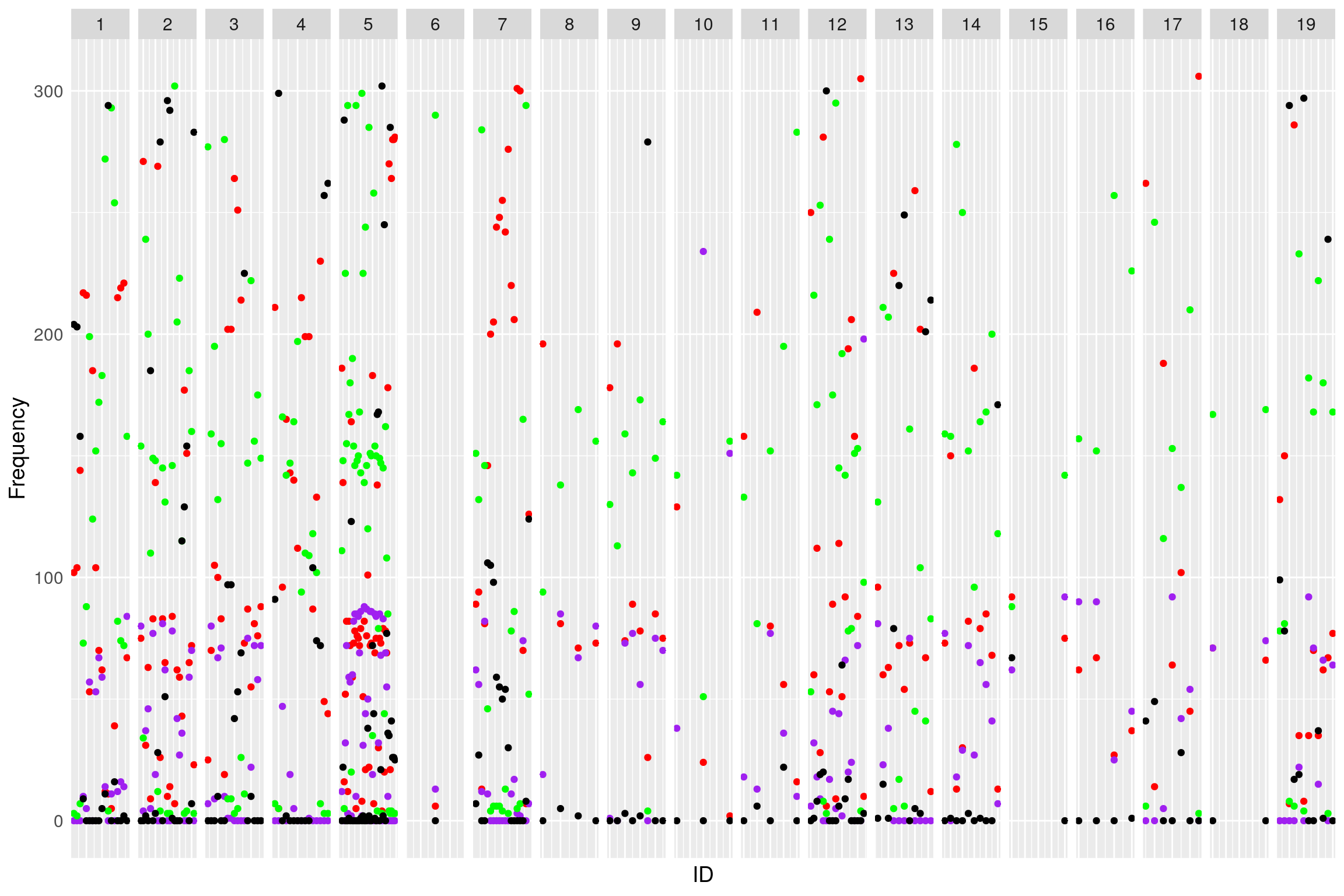
Genotype_distribution_post
# Choose who to drop. I chose A > H/4, B > H/4, H > (A+B)/2
dropm <- rownames(af)[af$A < af$H/4 | af$B < af$H/4 | af$H < (af$A+af$B)/2 | af$N > (af$A+af$B+af$H)]
WT144 <- drop.markers(WT144, dropm)
# Plot again
af <- NULL
for (chr in names(WT144$geno)){
  af <- rbind(af, data.frame(chr=chr,
                             A=colSums(WT144$geno[[chr]]$data == 1, na.rm = T),
                             H=colSums(WT144$geno[[chr]]$data == 2, na.rm = T),
                             B=colSums(WT144$geno[[chr]]$data == 3, na.rm = T),
                             N=colSums(is.na(WT144$geno[[chr]]$data))))
}
af$chr <- factor(af$chr, levels = names(WT144$geno))
af$ID <- 1:nrow(af)
#plot
genotype_distribution_post <- ggplot(af) +
  geom_point(aes(ID, A), color = "red") +
  geom_point(aes(ID, B), color="purple") +
  geom_point(aes(ID, H), color="green") +
  geom_point(aes(ID, N), color="black") +
  facet_grid(~chr, scales = "free") +
  ylab("Frequency") +
  theme(text = element_text(size = 14),
        axis.text.x = element_blank(),
        axis.ticks = element_blank())

print(genotype_distribution_post)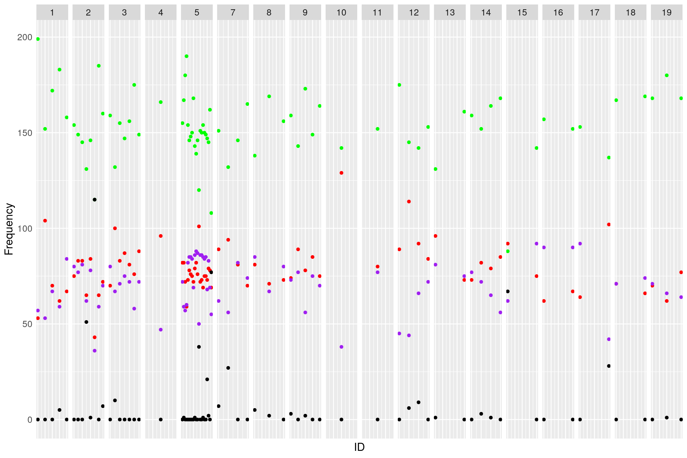
plotMap(WT144)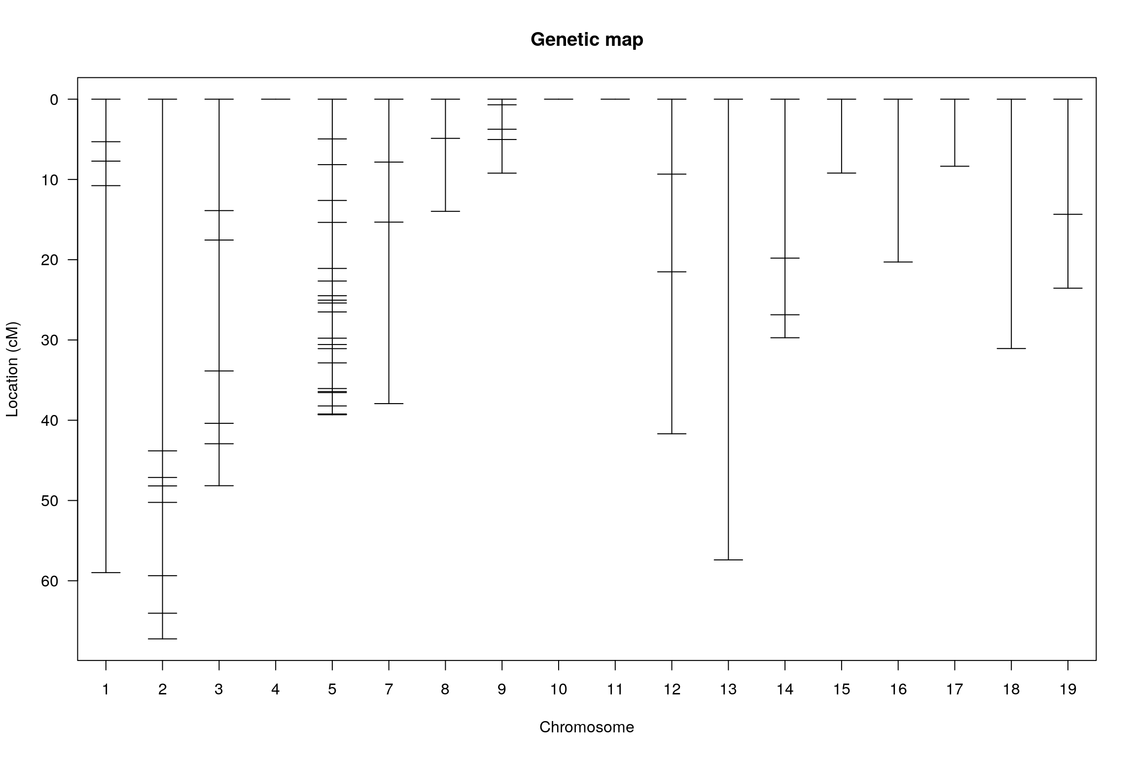
Process phenotype on the genotyped animals
#read data Report-12-27-2019.csv, It contains 2096 animals. The linear model performed by Asaf is based on 2096 animals. However, in the cross object WT144, 309 animals were genotyped. Asaf just extracted the coefficients for these 309 animals.
report <- readr::read_csv("data/Report-12-27-2019.csv") %>%
  dplyr::select(animal_name, gender, TotalDist, TestAge, test.no) %>%
  dplyr::mutate(across(c(gender, test.no), as.factor))
#plot TotalDist vs test age among 2096 animals
p1 <- ggplot(data = report,
             mapping = aes(x = TestAge, y = TotalDist, color = test.no)) +
  geom_point(aes(shape=gender)) +
  geom_smooth(method=lm)
print(p1)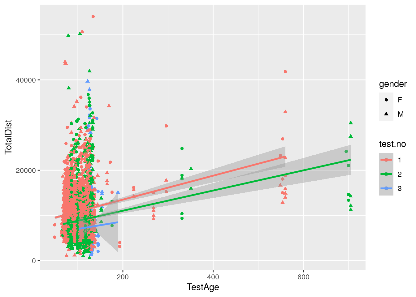
#plot TotalDist distribution across test.no among 2096 animals
p2 <- ggplot(data = report,
             mapping = aes(x = test.no, y = TotalDist, color = test.no)) +
  geom_boxplot()
print(p2)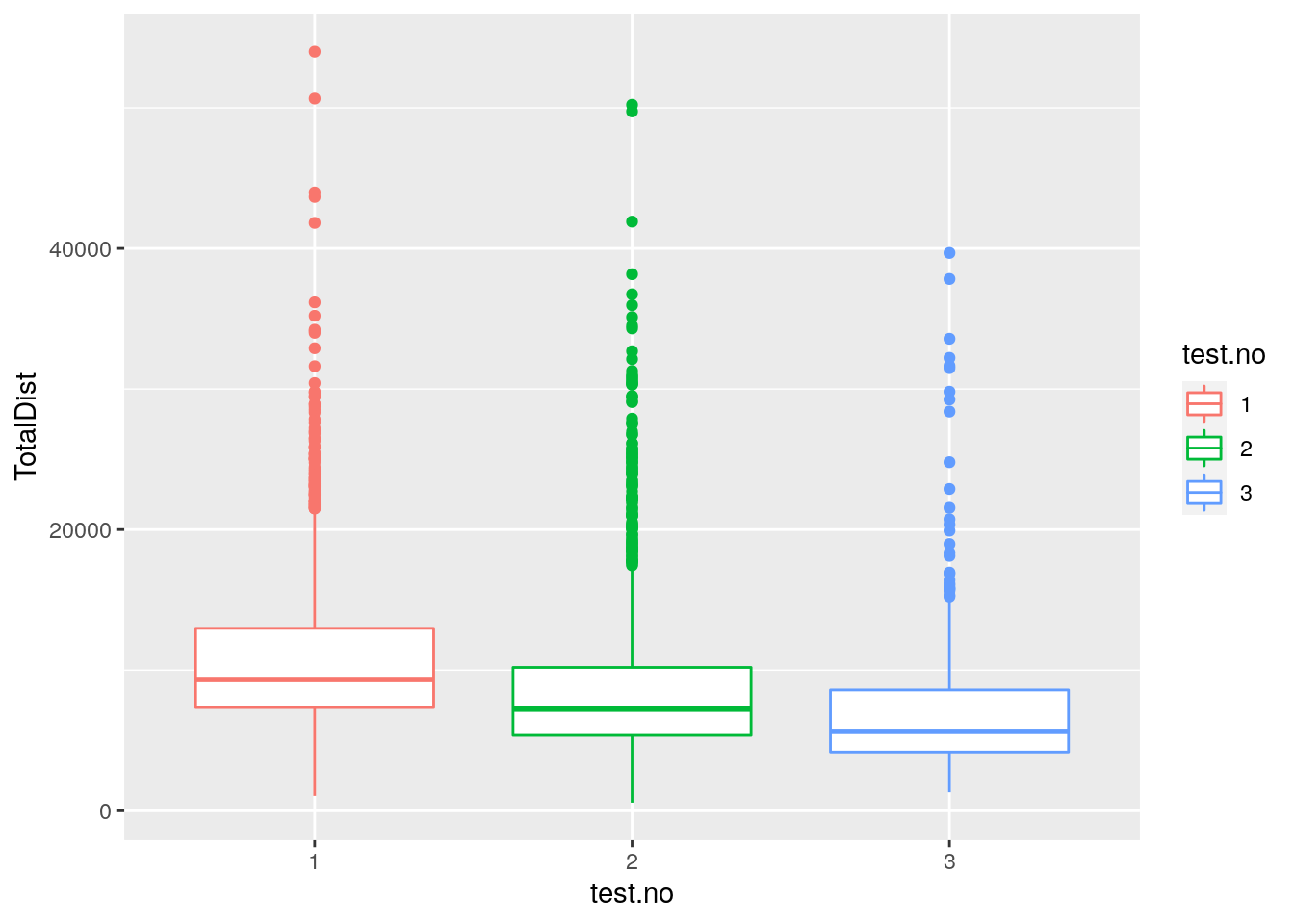
#plot histgram for TotalDist among 2096 animals
p3 <- ggplot(data = report,
             mapping = aes(x = TotalDist, fill = test.no)) +
  geom_histogram() +
  facet_grid(test.no ~ .)
print(p3)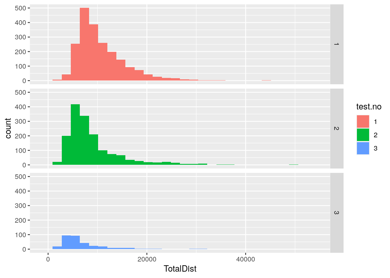
#plot histgram for TotalDist for genders with mean lines among 2096 animals
p4 <- ggplot(data = report,
             mapping = aes(x = TotalDist, fill = gender)) +
  geom_histogram()
print(p4)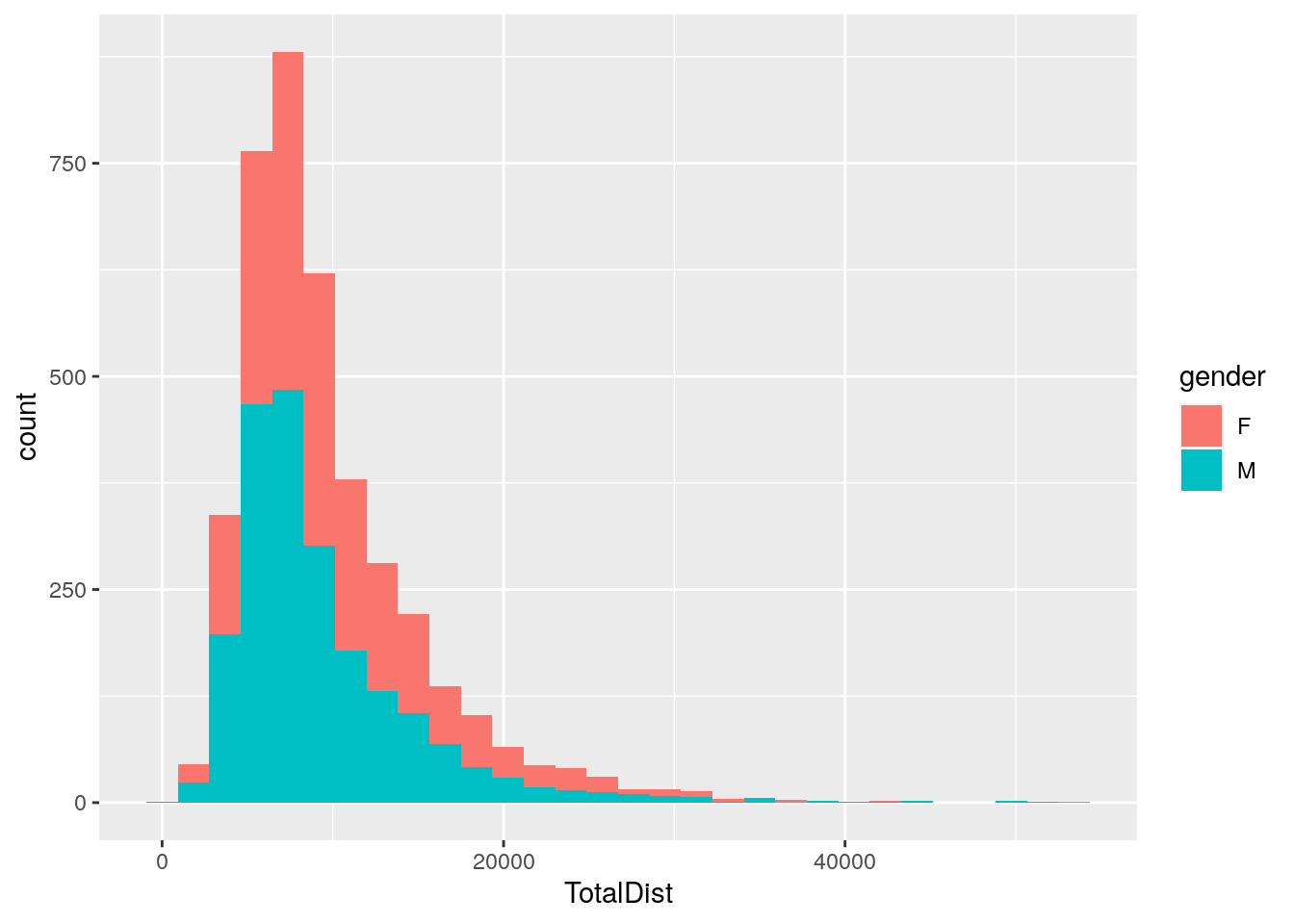
#model by Asaf using 2096 animals
anml <- lm(TotalDist ~ gender + animal_name * TestAge, data=report)
#coefs
coefs <- tibble(names = names(anml$coefficients), allvals = anml$coefficients) %>%
  filter(grepl("animal_name", names)) %>%
  # Add a column to indicate if it's the name or the interactions
  separate(names, c("animal_name", "interaction") ,sep=":")
coefs$interaction <- replace_na(coefs$interaction, "base")
coefs$animal_name <- gsub("animal_name", "", coefs$animal_name)
coefs <- pivot_wider(coefs, id_cols = animal_name, names_from = interaction, values_from = allvals)
rep_wide <- pivot_wider(report, names_from = test.no, values_from = c("TestAge", "TotalDist"))
table_all <- left_join(coefs, rep_wide, by="animal_name") %>% rename(AnimalName=animal_name, Gender=gender)

#histgram for base model by Asaf using 2096 animals
p5 <- ggplot(data = table_all,
             mapping = aes(x = base, fill = Gender)) +
  geom_histogram() +
  ggtitle("Histgram for base modeled from 2096 animals")
print(p5)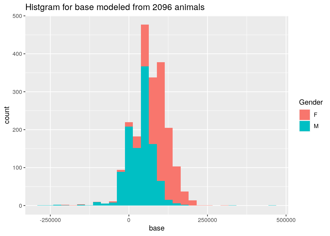
#read data Report-12-27-2019.csv and filter to the 309 animals which also have genotypes.
report <- readr::read_csv("data/Report-12-27-2019.csv") %>%
  dplyr::select(animal_name, gender, TotalDist, TestAge, test.no) %>%
  dplyr::filter(animal_name %in% WT144$pheno$AnimalName) %>% #filter to the animals with genotypes
  dplyr::mutate(across(c(gender, test.no), as.factor))
#plot TotalDist vs test age among 309 animals
p6 <- ggplot(data = report,
             mapping = aes(x = TestAge, y = TotalDist, color = test.no)) +
  geom_point(aes(shape=gender)) +
  geom_smooth(method=lm)
print(p6)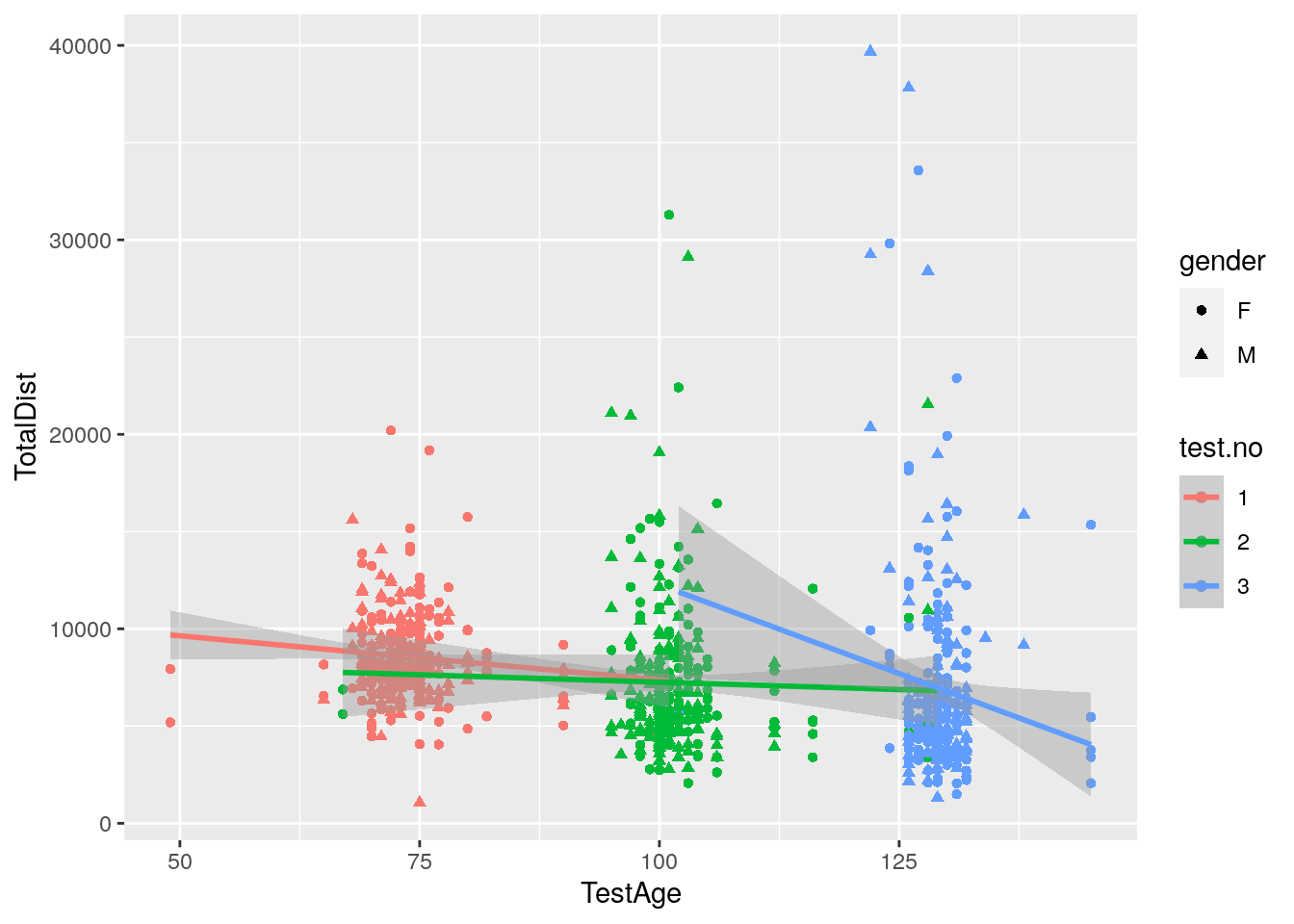
#plot TotalDist distribution across test.no among 309 animals
p7 <- ggplot(data = report,
             mapping = aes(x = test.no, y = TotalDist, color = test.no)) +
  geom_boxplot()
print(p7)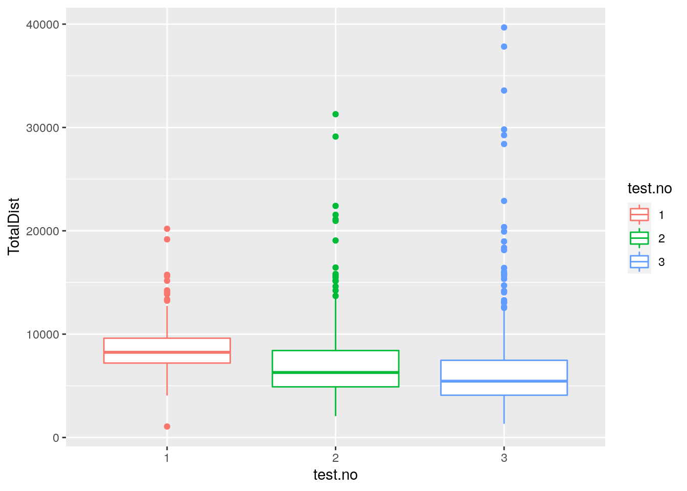
#plot histgram for TotalDist among 309 animals
p8 <- ggplot(data = report,
             mapping = aes(x = TotalDist, fill = test.no)) +
  geom_histogram() +
  facet_grid(test.no ~ .)
print(p8)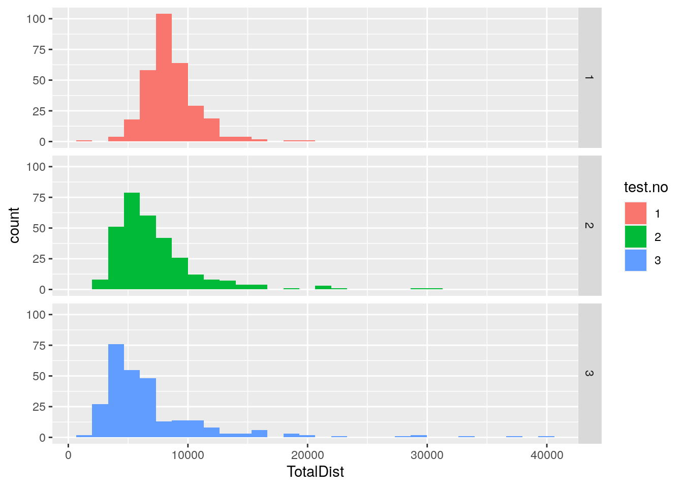
#plot histgram for TotalDist for genders with mean lines among 309 animals
p9 <- ggplot(data = report,
             mapping = aes(x = TotalDist, fill = gender)) +
  geom_histogram()
print(p9)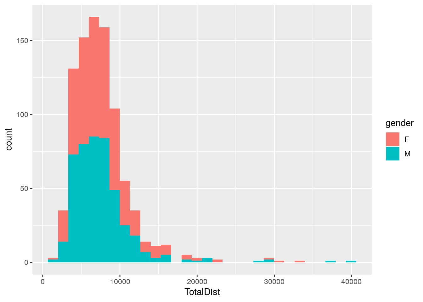
#From Asaf:
# I took the input file and ran lm with the formula: TotalDist ~ gender + animal_name * TestAge and extracted the coefficients for the animal alone and the interaction with age. For some reason the distribution of the animal coefficients alone is bi-modal."

# It is because the model by Asaf is based on 2096 animals, but the coefficients Asaf extracted is only for the animals with genotypes. 309 animals out of 2096 have genotypes. It resulted in a sampling bias. We should focus on the animals having both phenotype and genotype.

#model
anml <- lm(TotalDist ~ gender + animal_name * TestAge, data=report) # animal_name as a fixed effect
#coefs
coefs <- tibble(names = names(anml$coefficients), allvals = anml$coefficients) %>%
  filter(grepl("animal_name", names)) %>%
  # Add a column to indicate if it's the name or the interactions
  separate(names, c("animal_name", "interaction") ,sep=":")
coefs$interaction <- replace_na(coefs$interaction, "base")# make coefficient of animal_name as base
coefs$animal_name <- gsub("animal_name", "", coefs$animal_name)
coefs <- pivot_wider(coefs, id_cols = animal_name, names_from = interaction, values_from = allvals)
rep_wide <- pivot_wider(report, names_from = test.no, values_from = c("TestAge", "TotalDist"))
table_all <- left_join(coefs, rep_wide, by="animal_name") %>% rename(AnimalName=animal_name, Gender=gender)

#add table_all to the phenotype df in WT144
WT144$pheno <- left_join(WT144$pheno, table_all[, 1:3], by = "AnimalName")
#phenotype distribution
#plot histgram for base.x, which is calculated from the 2096 animals of report data/Report-12-27-2019.csv by Asaf
plotPheno(WT144, pheno.col=3, xlab = "base.x", main = "")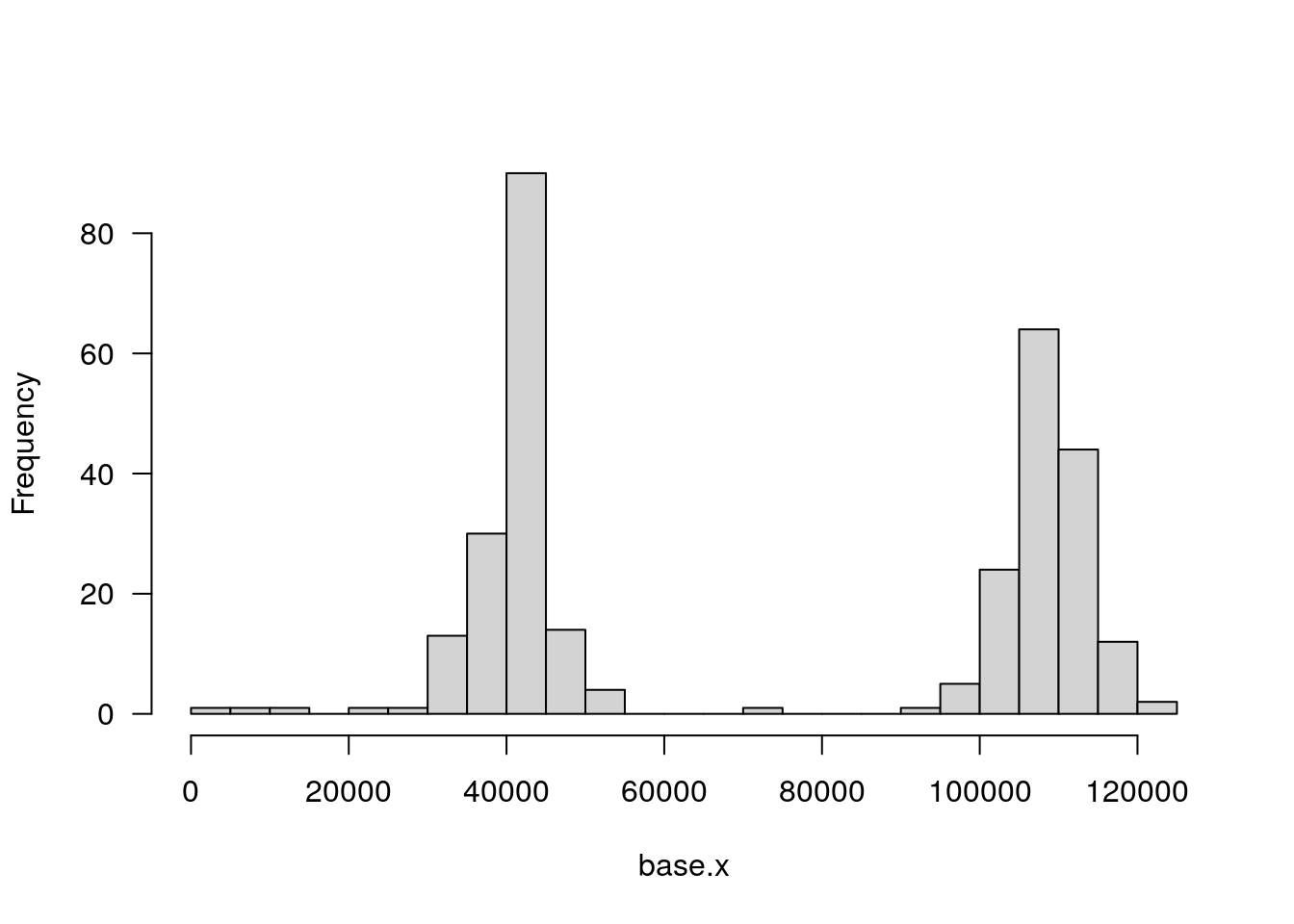
#plot base.x  by gender
p10 <- ggplot(data = WT144$pheno,
             mapping = aes(x = base.x, fill = Gender)) +
  geom_histogram()
print(p10)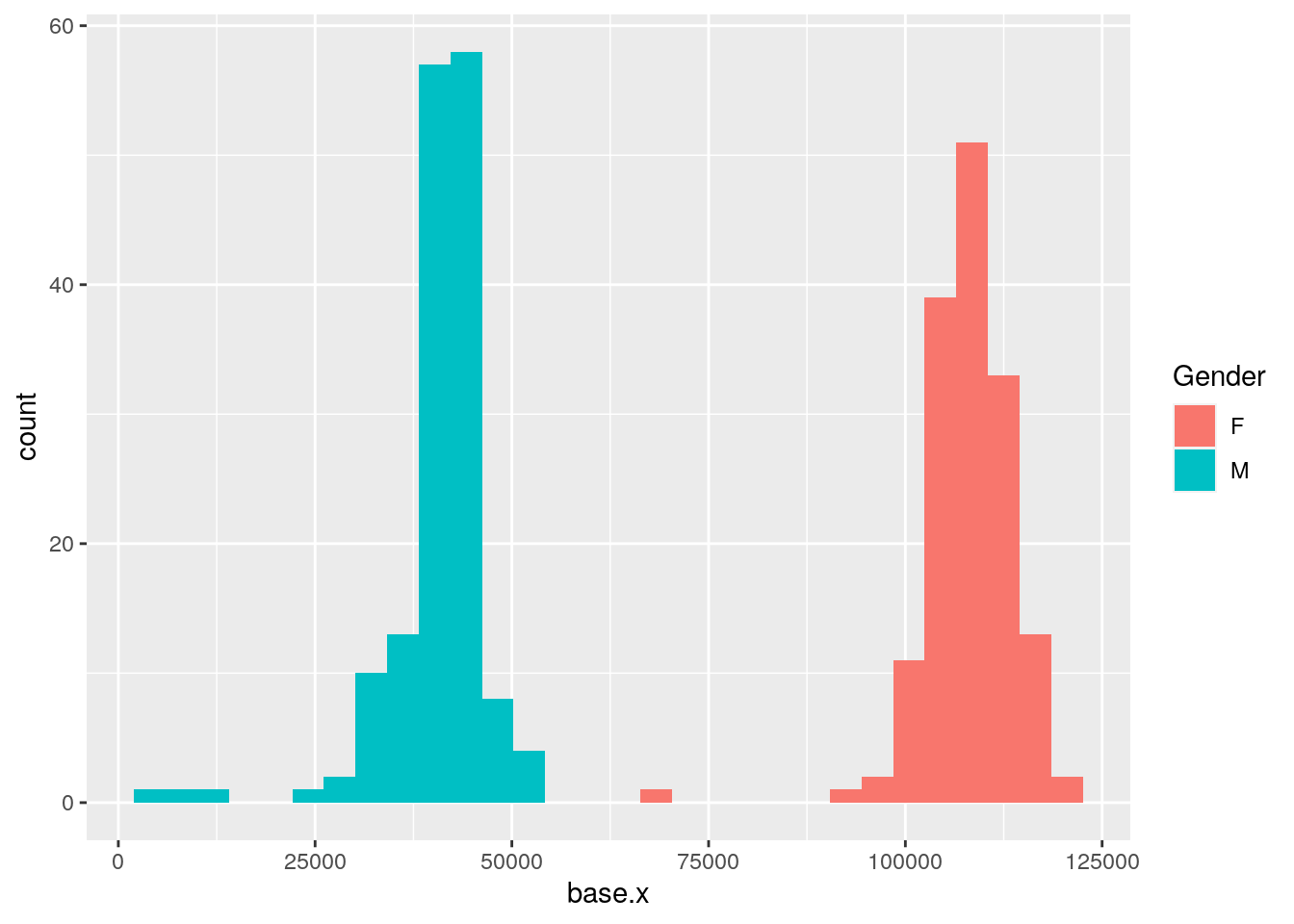
#plot base.x  vs TestAge.x
p11 <- ggplot(data = WT144$pheno,
             mapping = aes(x = TestAge.x, y = base.x, color = Gender)) +
  geom_point()+
  geom_smooth(method=lm)
print(p11)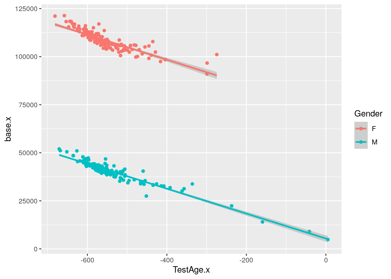
#plot histgram for TestAge.x, which is calculated from the 2096 animals of report data/Report-12-27-2019.csv
plotPheno(WT144, pheno.col=4, xlab = "TestAge.x", main = "")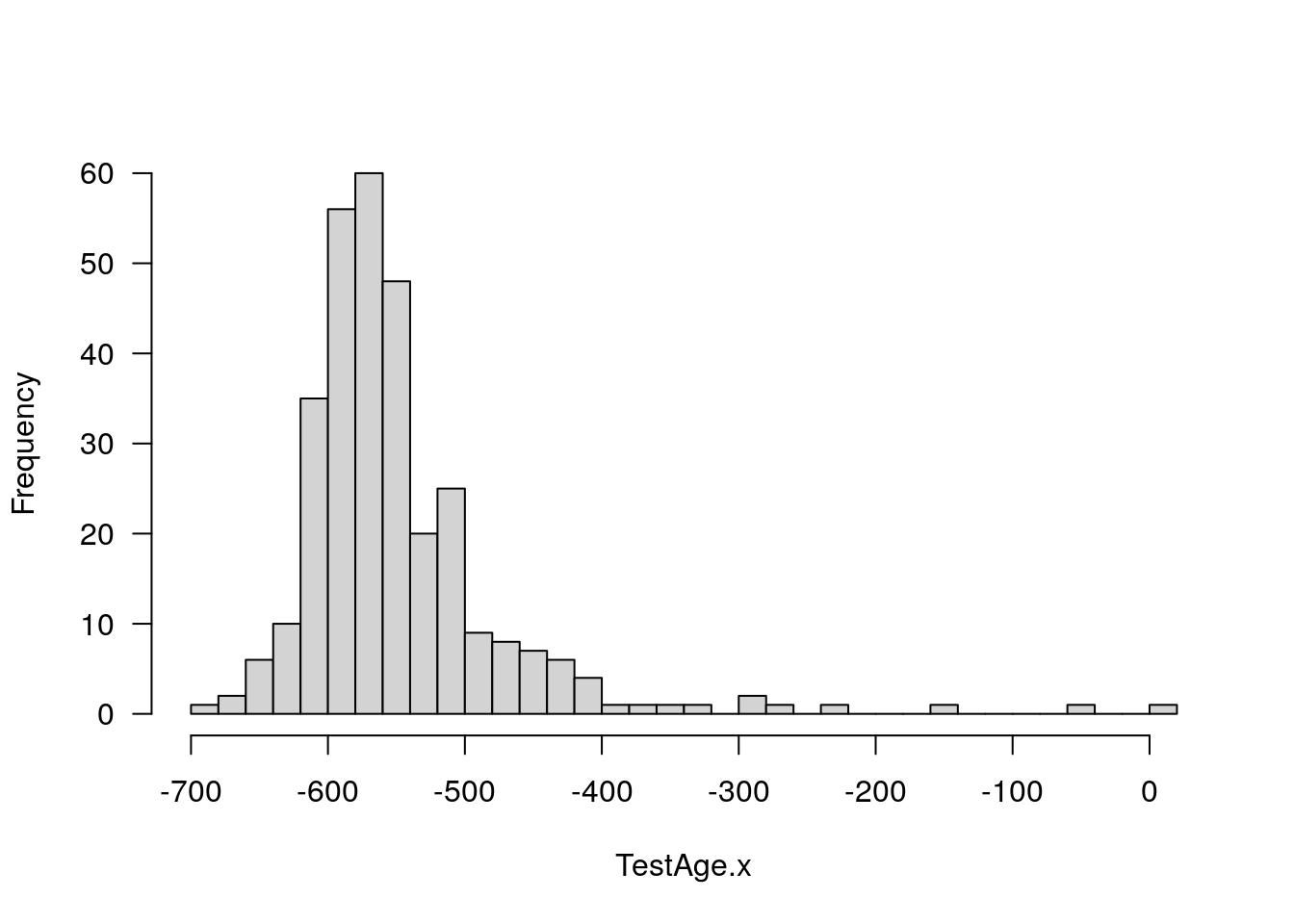
plotPheno(WT144, pheno.col=9, xlab = "TotalDist_1", main = "")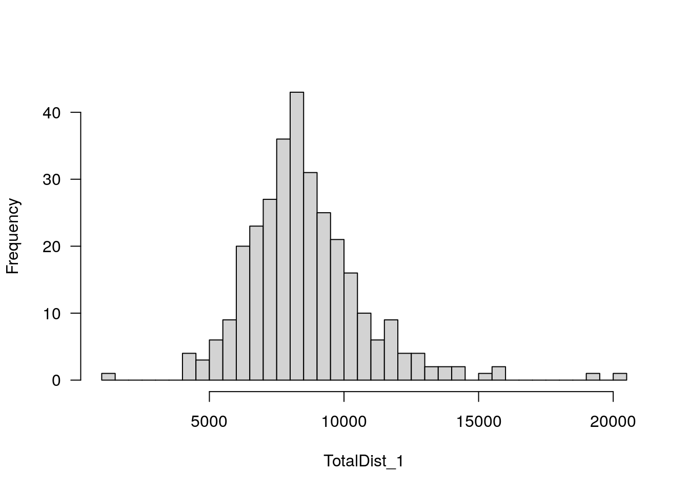
plotPheno(WT144, pheno.col=10, xlab = "TotalDist_2", main = "")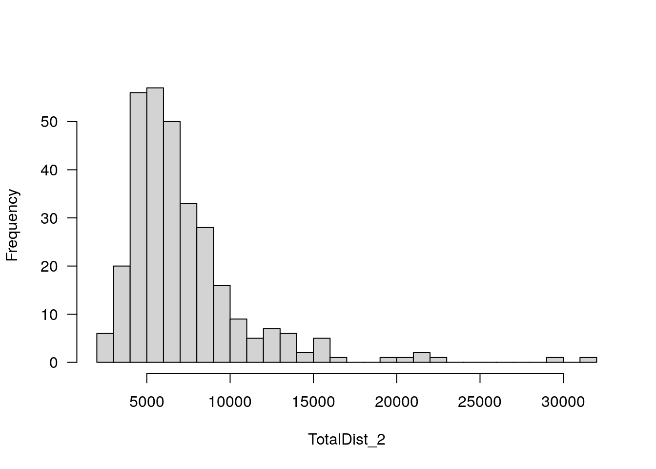
plotPheno(WT144, pheno.col=11, xlab = "TotalDist_3", main = "")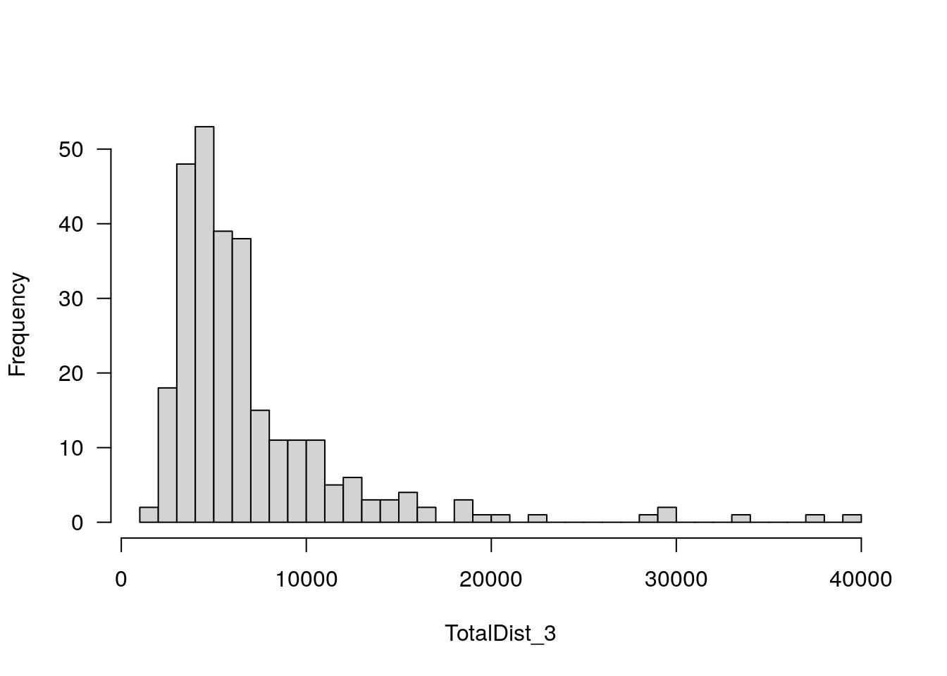
#plot histgram for base.y, which is calculated from the animals having both genotypes and phenotypes
plotPheno(WT144, pheno.col=12, xlab = "base.y", main = "")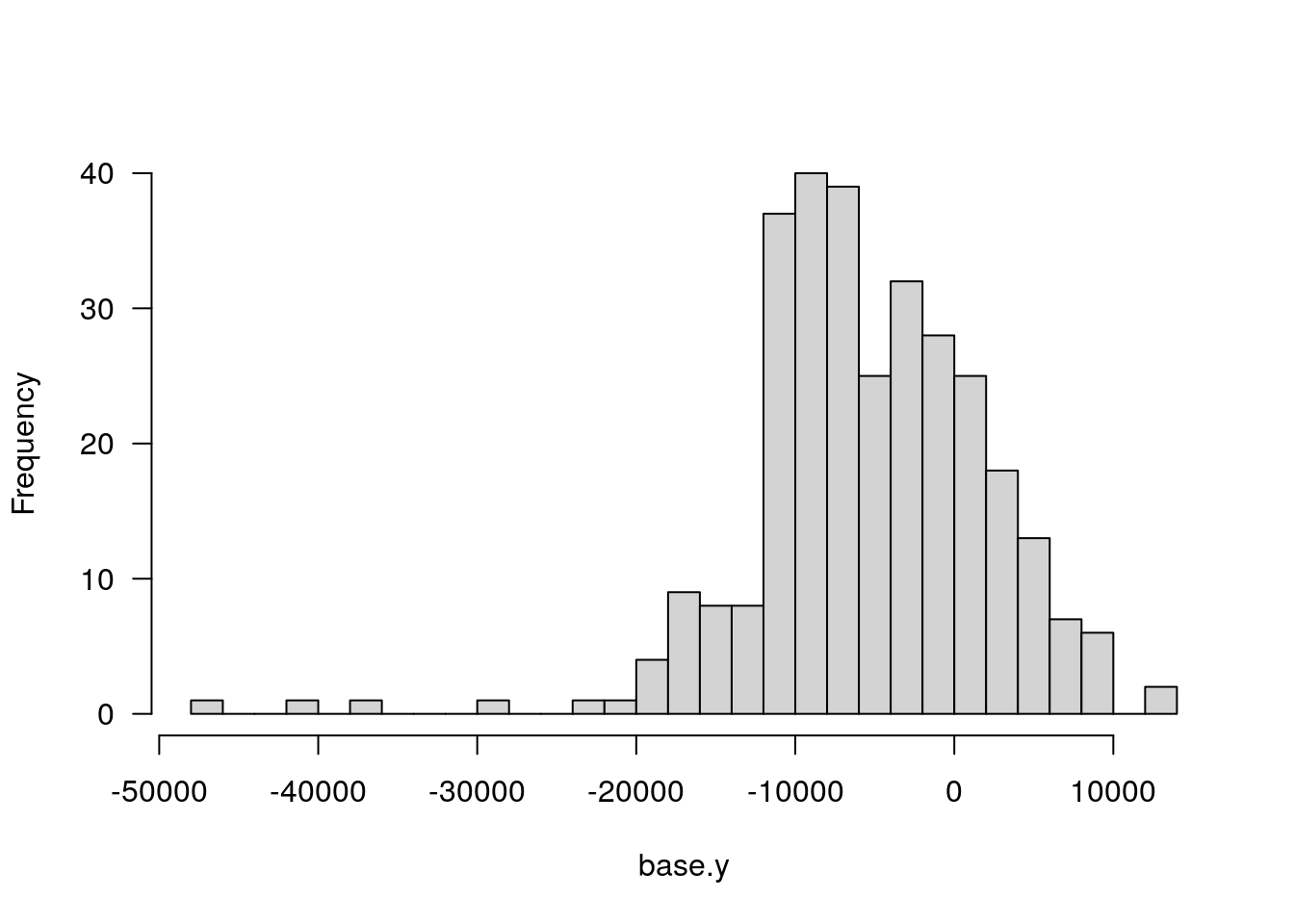
#plot base.y  by gender
p12 <- ggplot(data = WT144$pheno,
             mapping = aes(x = base.y, fill = Gender)) +
  geom_histogram()
print(p12)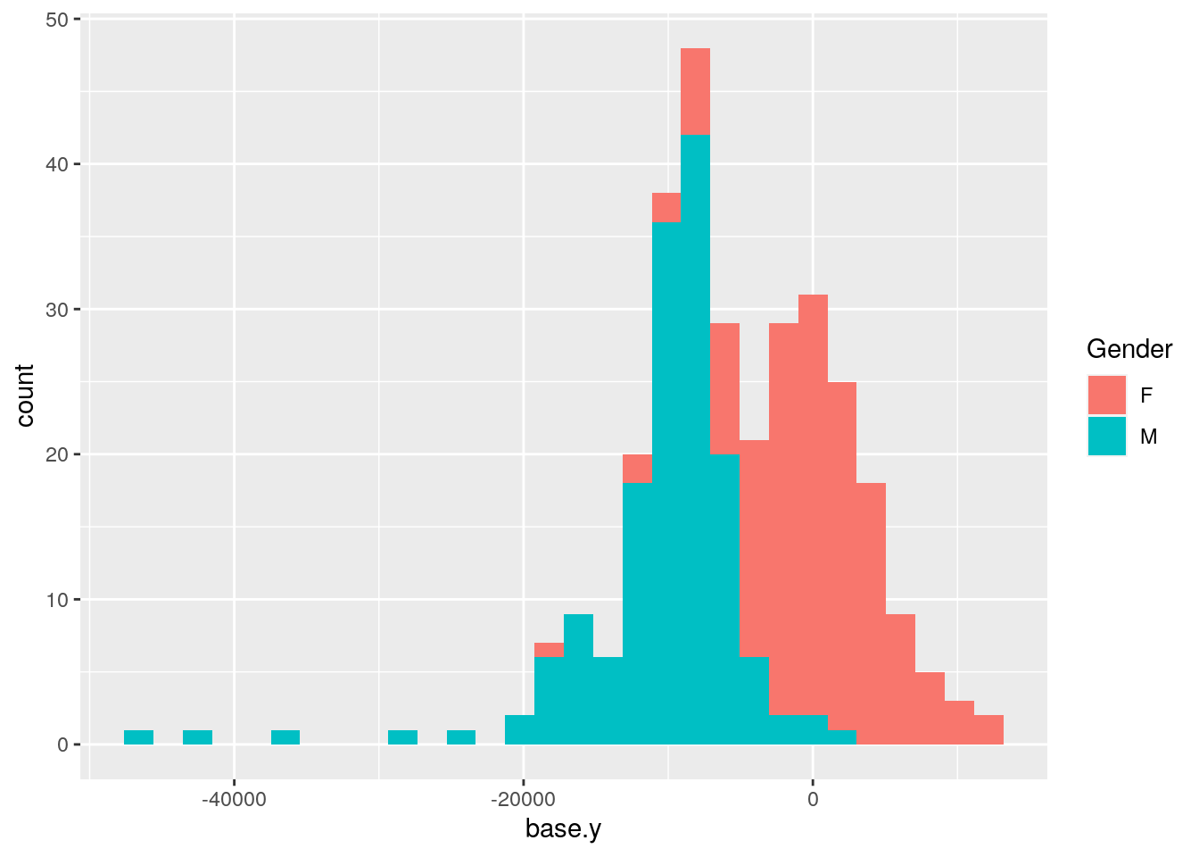
#plot base.y vs TestAge.y
p13 <- ggplot(data = WT144$pheno,
             mapping = aes(x = TestAge.y, y = base.y, color = Gender)) +
  geom_point()+
  geom_smooth(method=lm)
print(p13)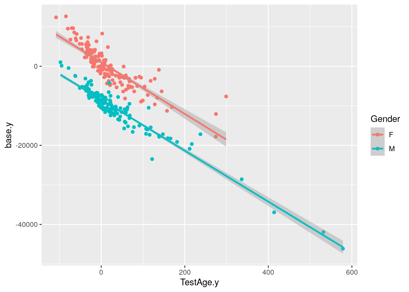
#plot histgram for TestAge.y, which is calculated from the animals having both genotypes and phenotypes
plotPheno(WT144, pheno.col=13, xlab = "TestAge.y", main = "")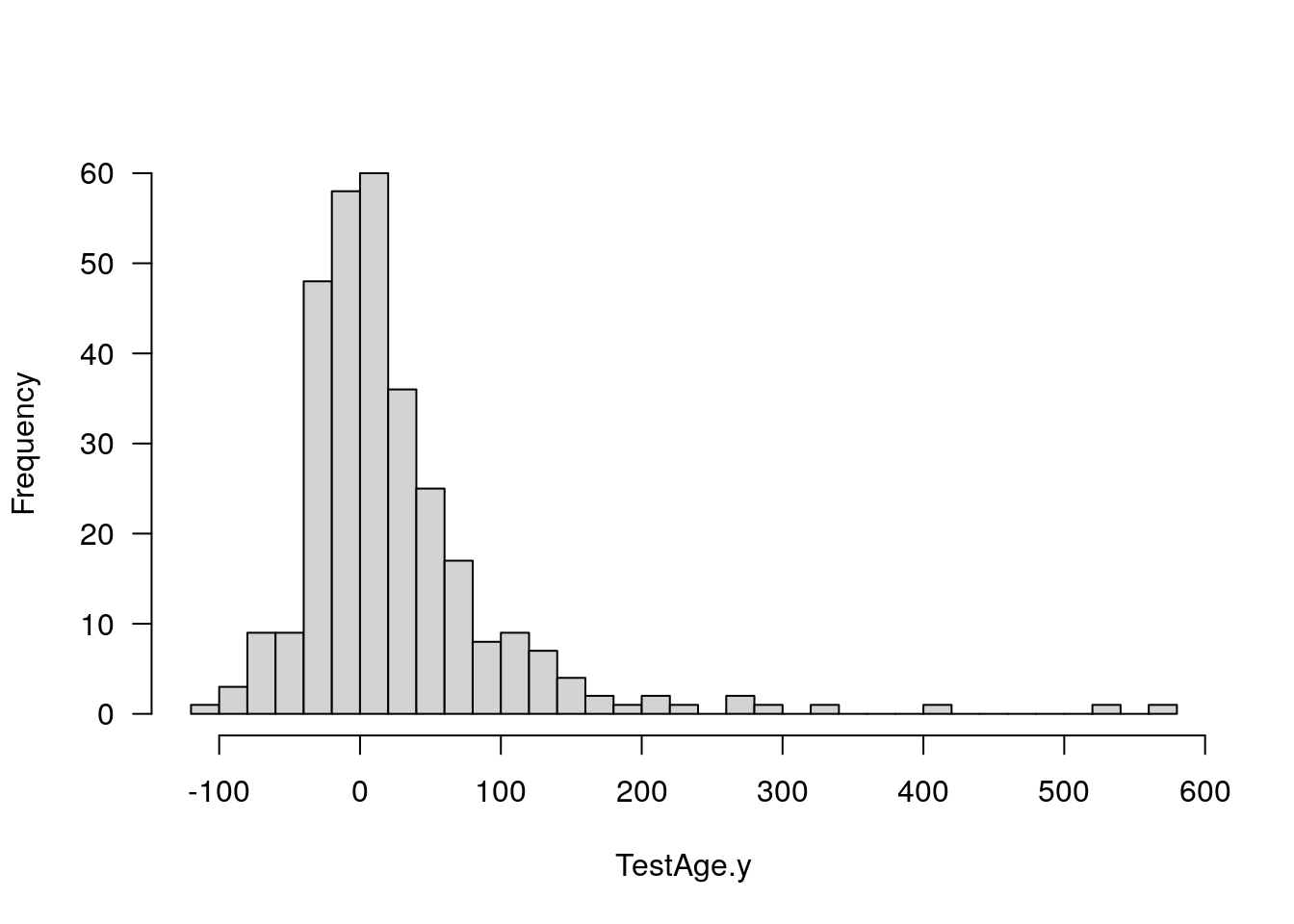
#a random intercept for each animal,
#and a random slope of TestAge for each animal
#This allows both the intercept and the slope of TestAge to vary across animals
res <- lmer(TotalDist ~ TestAge + (1 + TestAge|animal_name),
              data = report)
summary(res)
Linear mixed model fit by REML. t-tests use Satterthwaite's method [
lmerModLmerTest]
Formula: TotalDist ~ TestAge + (1 + TestAge | animal_name)
Data: report
REML criterion at convergence: 16596.9
Scaled residuals:
Min 1Q Median 3Q Max
-3.5368 -0.4085 -0.0295 0.3694 3.7790
Random effects:
Groups Name Variance Std.Dev. Corr
animal_name (Intercept) 12321442 3510.2
TestAge 4265 65.3 -0.96
Residual 2173666 1474.3
Number of obs: 898, groups: animal_name, 309
Fixed effects:
Estimate Std. Error df t value Pr(>|t|)
(Intercept) 10338.640 302.752 321.518 34.149 < 2e-16 ***
TestAge -26.522 4.333 317.190 -6.121 2.75e-09 ***
---
Signif. codes: 0 '***' 0.001 '**' 0.01 '*' 0.05 '.' 0.1 ' ' 1
Correlation of Fixed Effects:
(Intr)
TestAge -0.918
optimizer (nloptwrap) convergence code: 0 (OK)
Model failed to converge with max|grad| = 1.58588 (tol = 0.002, component 1)
Model is nearly unidentifiable: very large eigenvalue
- Rescale variables?confint(res, level = 0.95, method = "Wald") 2.5 % 97.5 %
.sig01 NA NA
.sig02 NA NA
.sig03 NA NA
.sigma NA NA
(Intercept) 9745.25700 10932.02232
TestAge -35.01462 -18.02879#there is strong evidence that TestAge significantly decreased TotalDist.
res.std <- resid(res)/sd(resid(res))
plot(res.std, ylab="Standardized Residuals")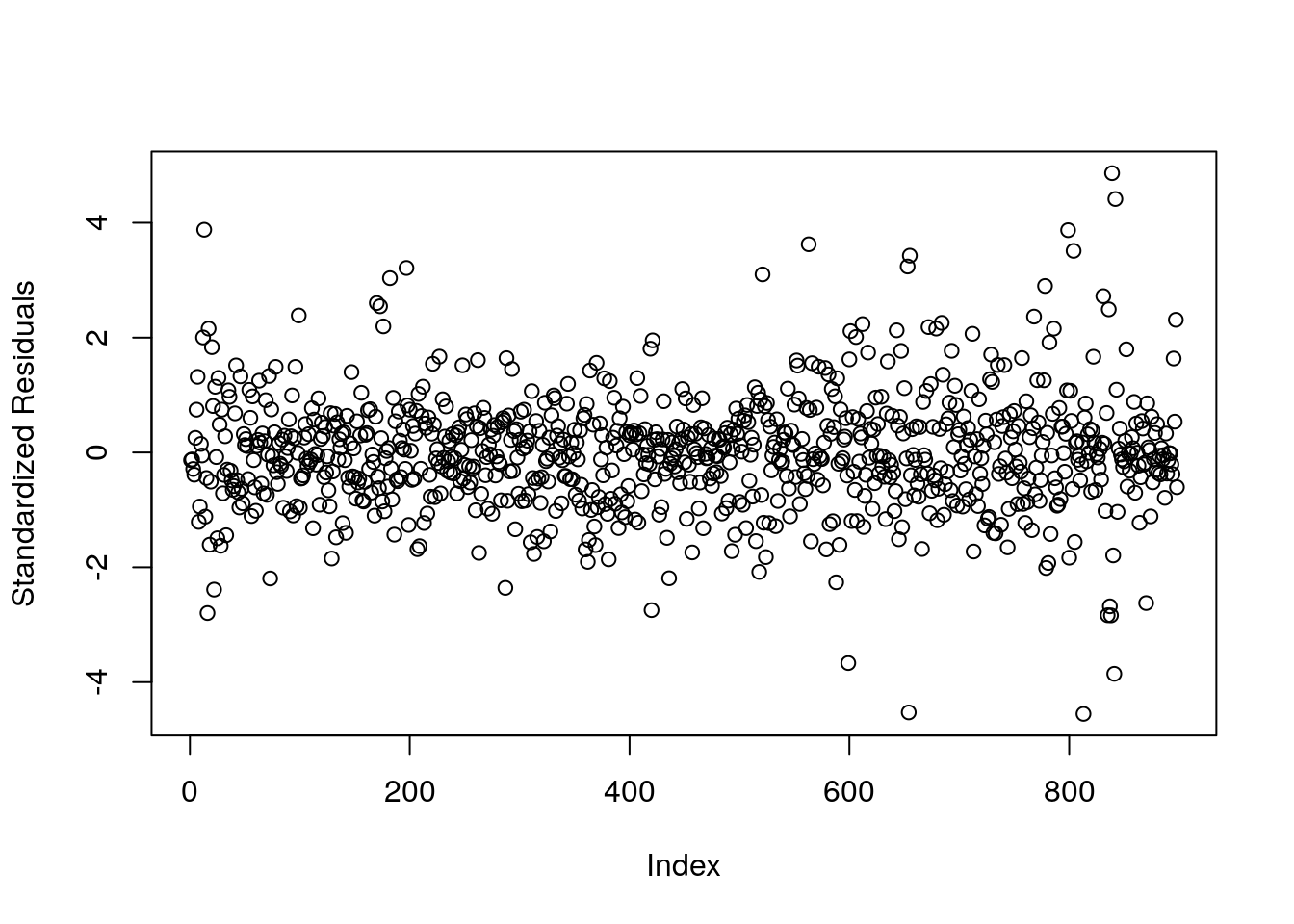
ggplot(as.data.frame(res.std), aes(sample = res.std)) +
  geom_qq() +
  geom_qq_line()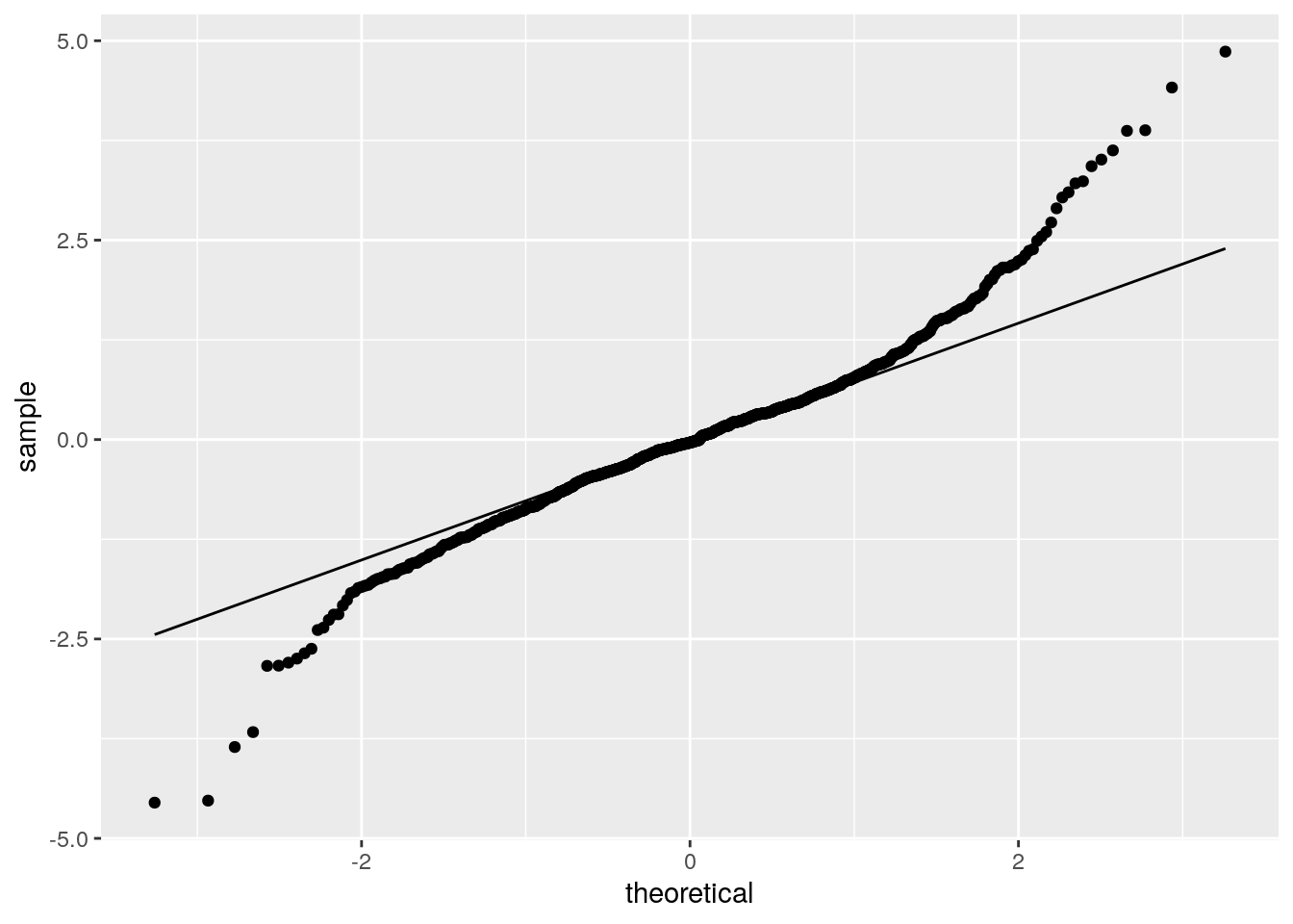
#to get the fitted Intercept and Slope
TotalDist_animal <- coef(res)$animal_name
colnames(TotalDist_animal) <- c("Intercept", "Slope")
TotalDist_animal$AnimalName<-rownames(TotalDist_animal)

#add TotalDist_animal to the phenotype df in WT144
WT144$pheno <- left_join(WT144$pheno, TotalDist_animal, by = "AnimalName")
plotPheno(WT144, pheno.col=14, xlab = "")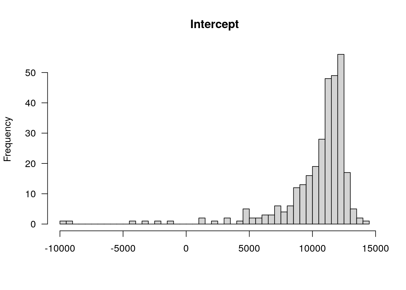
plotPheno(WT144, pheno.col=15, xlab = "")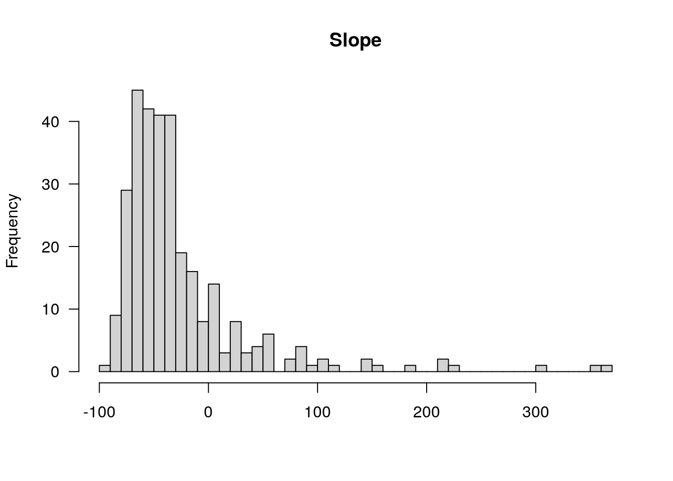
Run qtl
#run qtl
print(summary(WT144))
F2 intercross
No. individuals: 309
No. phenotypes: 15
Percent phenotyped: 100 100 100 99.7 100 100 99.7 90.9 100 99.7 90.9 99.4
99.4 100 100
No. chromosomes: 18
Autosomes: 1 2 3 4 5 7 8 9 10 11 12 13 14 15 16 17 18 19
Total markers: 78
No. markers: 5 8 7 1 22 4 3 5 1 1 4 2 4 2 2 2 2 3
Percent genotyped: 98
Genotypes (%): AA:25.9 AB:50.7 BB:23.3 not BB:0.0 not AA:0.0 WT144 <- drop.nullmarkers(WT144)
covars <- model.matrix(~ Gender, WT144$pheno)[,-1]
#idx
idx <- c(3,4,9:15)
out.mr <- operm <- st <- list()
#loop for each pheno
for (i in 1:length(idx)){
out.mr[[i]] <- scanone(WT144, pheno.col=idx[[i]], method="mr", addcovar=covars)
out.mr[[i]]$lod[is.infinite(out.mr[[i]]$lod)]=0
print(summary(out.mr[[i]]))
#operm
operm[[i]] <-scanone(WT144, pheno.col=idx[[i]], n.perm=1000, method="mr", addcovar=covars)
print(summary(operm[[i]]))
#scantwo
st[[i]] <- scantwo(WT144, pheno.col = idx[[i]], method="mr")
} chr pos lod
chr1-65643621-.-C-A 1 33.25 1.1141
chr2-7018694-.-G-T 2 3.85 0.9696
chr3-59218564-.-T-A 3 29.01 1.3635
chr4-32821418-.-C-T 4 14.44 1.6091
chr5-136332619-.-C-A 5 75.98 11.1313
chr7-112510032-.-A-T 7 58.79 0.4425
chr8-112465004-.-G-A 8 58.61 0.2427
chr9-71739608-.-T-A 9 39.90 0.6909
chr10-24134777-.-A-T 10 11.46 0.7016
chr11-96730656-.-A-G 11 60.12 0.0244
chr12-43136399-.-A-T 12 19.48 1.7403
chr13-115031098-.-T-C 13 64.63 1.0510
chr14-69691477-.-G-T 14 36.07 4.4517
chr15-58605950-.-C-G 15 25.02 1.0287
chr16-75648687-.-G-A 16 43.33 0.8763
chr17-61305603-.-G-A 17 31.92 0.5478
chr18-51300216-.-T-A 18 27.94 0.4609
chr19-53469239-.-A-G 19 48.00 1.5870
Permutation 20
Permutation 40
Permutation 60
Permutation 80
Permutation 100
Permutation 120
Permutation 140
Permutation 160
Permutation 180
Permutation 200
Permutation 220
Permutation 240
Permutation 260
Permutation 280
Permutation 300
Permutation 320
Permutation 340
Permutation 360
Permutation 380
Permutation 400
Permutation 420
Permutation 440
Permutation 460
Permutation 480
Permutation 500
Permutation 520
Permutation 540
Permutation 560
Permutation 580
Permutation 600
Permutation 620
Permutation 640
Permutation 660
Permutation 680
Permutation 700
Permutation 720
Permutation 740
Permutation 760
Permutation 780
Permutation 800
Permutation 820
Permutation 840
Permutation 860
Permutation 880
Permutation 900
Permutation 920
Permutation 940
Permutation 960
Permutation 980
Permutation 1000
LOD thresholds (1000 permutations)
lod
5% 2.97
10% 2.71
 --Running scanone
 --Running scantwo
 (1,1)
 (1,2)
 (1,3)
 (1,4)
 (1,5)
 (1,7)
 (1,8)
 (1,9)
 (1,10)
 (1,11)
 (1,12)
 (1,13)
 (1,14)
 (1,15)
 (1,16)
 (1,17)
 (1,18)
 (1,19)
 (2,2)
 (2,3)
 (2,4)
 (2,5)
 (2,7)
 (2,8)
 (2,9)
 (2,10)
 (2,11)
 (2,12)
 (2,13)
 (2,14)
 (2,15)
 (2,16)
 (2,17)
 (2,18)
 (2,19)
 (3,3)
 (3,4)
 (3,5)
 (3,7)
 (3,8)
 (3,9)
 (3,10)
 (3,11)
 (3,12)
 (3,13)
 (3,14)
 (3,15)
 (3,16)
 (3,17)
 (3,18)
 (3,19)
 (4,4)
 (4,5)
 (4,7)
 (4,8)
 (4,9)
 (4,10)
 (4,11)
 (4,12)
 (4,13)
 (4,14)
 (4,15)
 (4,16)
 (4,17)
 (4,18)
 (4,19)
 (5,5)
 (5,7)
 (5,8)
 (5,9)
 (5,10)
 (5,11)
 (5,12)
 (5,13)
 (5,14)
 (5,15)
 (5,16)
 (5,17)
 (5,18)
 (5,19)
 (7,7)
 (7,8)
 (7,9)
 (7,10)
 (7,11)
 (7,12)
 (7,13)
 (7,14)
 (7,15)
 (7,16)
 (7,17)
 (7,18)
 (7,19)
 (8,8)
 (8,9)
 (8,10)
 (8,11)
 (8,12)
 (8,13)
 (8,14)
 (8,15)
 (8,16)
 (8,17)
 (8,18)
 (8,19)
 (9,9)
 (9,10)
 (9,11)
 (9,12)
 (9,13)
 (9,14)
 (9,15)
 (9,16)
 (9,17)
 (9,18)
 (9,19)
 (10,10)
 (10,11)
 (10,12)
 (10,13)
 (10,14)
 (10,15)
 (10,16)
 (10,17)
 (10,18)
 (10,19)
 (11,11)
 (11,12)
 (11,13)
 (11,14)
 (11,15)
 (11,16)
 (11,17)
 (11,18)
 (11,19)
 (12,12)
 (12,13)
 (12,14)
 (12,15)
 (12,16)
 (12,17)
 (12,18)
 (12,19)
 (13,13)
 (13,14)
 (13,15)
 (13,16)
 (13,17)
 (13,18)
 (13,19)
 (14,14)
 (14,15)
 (14,16)
 (14,17)
 (14,18)
 (14,19)
 (15,15)
 (15,16)
 (15,17)
 (15,18)
 (15,19)
 (16,16)
 (16,17)
 (16,18)
 (16,19)
 (17,17)
 (17,18)
 (17,19)
 (18,18)
 (18,19)
 (19,19)
Warning in checkcovar(cross, pheno.col, addcovar, intcovar, perm.strata, : Dropping 1 individuals with missing phenotypes. chr pos lod
chr1-65643621-.-C-A 1 33.25 1.929
chr2-7018694-.-G-T 2 3.85 1.116
chr3-59218564-.-T-A 3 29.01 1.451
chr4-32821418-.-C-T 4 14.44 1.007
chr5-136332619-.-C-A 5 75.98 21.390
chr7-112510032-.-A-T 7 58.79 0.114
chr8-99395759-.-T-C 8 49.52 0.273
chr9-69415567-.-T-A 9 38.63 0.662
chr10-24134777-.-A-T 10 11.46 1.668
chr11-96730656-.-A-G 11 60.12 0.217
chr12-43136399-.-A-T 12 19.48 1.922
chr13-115031098-.-T-C 13 64.63 1.615
chr14-69691477-.-G-T 14 36.07 5.370
chr15-58605950-.-C-G 15 25.02 0.362
chr16-32593683-.-A-G 16 23.04 0.519
chr17-69219676-.-G-A 17 40.27 0.447
chr18-51300216-.-T-A 18 27.94 0.219
chr19-53469239-.-A-G 19 48.00 0.760Warning in checkcovar(cross, pheno.col, addcovar, intcovar, perm.strata, : Dropping 1 individuals with missing phenotypes.Permutation 20
Permutation 40
Permutation 60
Permutation 80
Permutation 100
Permutation 120
Permutation 140
Permutation 160
Permutation 180
Permutation 200
Permutation 220
Permutation 240
Permutation 260
Permutation 280
Permutation 300
Permutation 320
Permutation 340
Permutation 360
Permutation 380
Permutation 400
Permutation 420
Permutation 440
Permutation 460
Permutation 480
Permutation 500
Permutation 520
Permutation 540
Permutation 560
Permutation 580
Permutation 600
Permutation 620
Permutation 640
Permutation 660
Permutation 680
Permutation 700
Permutation 720
Permutation 740
Permutation 760
Permutation 780
Permutation 800
Permutation 820
Permutation 840
Permutation 860
Permutation 880
Permutation 900
Permutation 920
Permutation 940
Permutation 960
Permutation 980
Permutation 1000
LOD thresholds (1000 permutations)
lod
5% 3.01
10% 2.72Warning in checkcovar(cross, pheno.col, addcovar, intcovar, perm.strata, : Dropping 1 individuals with missing phenotypes. --Running scanone
--Running scantwo
(1,1)
(1,2)
(1,3)
(1,4)
(1,5)
(1,7)
(1,8)
(1,9)
(1,10)
(1,11)
(1,12)
(1,13)
(1,14)
(1,15)
(1,16)
(1,17)
(1,18)
(1,19)
(2,2)
(2,3)
(2,4)
(2,5)
(2,7)
(2,8)
(2,9)
(2,10)
(2,11)
(2,12)
(2,13)
(2,14)
(2,15)
(2,16)
(2,17)
(2,18)
(2,19)
(3,3)
(3,4)
(3,5)
(3,7)
(3,8)
(3,9)
(3,10)
(3,11)
(3,12)
(3,13)
(3,14)
(3,15)
(3,16)
(3,17)
(3,18)
(3,19)
(4,4)
(4,5)
(4,7)
(4,8)
(4,9)
(4,10)
(4,11)
(4,12)
(4,13)
(4,14)
(4,15)
(4,16)
(4,17)
(4,18)
(4,19)
(5,5)
(5,7)
(5,8)
(5,9)
(5,10)
(5,11)
(5,12)
(5,13)
(5,14)
(5,15)
(5,16)
(5,17)
(5,18)
(5,19)
(7,7)
(7,8)
(7,9)
(7,10)
(7,11)
(7,12)
(7,13)
(7,14)
(7,15)
(7,16)
(7,17)
(7,18)
(7,19)
(8,8)
(8,9)
(8,10)
(8,11)
(8,12)
(8,13)
(8,14)
(8,15)
(8,16)
(8,17)
(8,18)
(8,19)
(9,9)
(9,10)
(9,11)
(9,12)
(9,13)
(9,14)
(9,15)
(9,16)
(9,17)
(9,18)
(9,19)
(10,10)
(10,11)
(10,12)
(10,13)
(10,14)
(10,15)
(10,16)
(10,17)
(10,18)
(10,19)
(11,11)
(11,12)
(11,13)
(11,14)
(11,15)
(11,16)
(11,17)
(11,18)
(11,19)
(12,12)
(12,13)
(12,14)
(12,15)
(12,16)
(12,17)
(12,18)
(12,19)
(13,13)
(13,14)
(13,15)
(13,16)
(13,17)
(13,18)
(13,19)
(14,14)
(14,15)
(14,16)
(14,17)
(14,18)
(14,19)
(15,15)
(15,16)
(15,17)
(15,18)
(15,19)
(16,16)
(16,17)
(16,18)
(16,19)
(17,17)
(17,18)
(17,19)
(18,18)
(18,19)
(19,19)
chr pos lod
chr1-79823528-.-A-G 1 41.0 0.547
chr2-137498061-.-T-A 2 67.9 3.383
chr3-145286160-.-C-A 3 69.4 1.454
chr4-32821418-.-C-T 4 14.4 0.368
chr5-136332619-.-C-A 5 76.0 12.517
chr7-112510032-.-A-T 7 58.8 0.542
chr8-91986173-.-T-C 8 44.6 0.557
chr9-65857475-.-T-C 9 35.6 0.577
chr10-24134777-.-A-T 10 11.5 1.638
chr11-96730656-.-A-G 11 60.1 0.282
chr12-69197484-.-C-A 12 28.8 0.472
chr13-115031098-.-T-C 13 64.6 0.993
chr14-62407765-.-T-A 14 33.2 4.482
chr15-58605950-.-C-G 15 25.0 0.879
chr16-75648687-.-G-A 16 43.3 0.258
chr17-69219676-.-G-A 17 40.3 0.775
chr18-51300216-.-T-A 18 27.9 0.174
chr19-29815794-.-A-T 19 24.5 0.521
Permutation 20
Permutation 40
Permutation 60
Permutation 80
Permutation 100
Permutation 120
Permutation 140
Permutation 160
Permutation 180
Permutation 200
Permutation 220
Permutation 240
Permutation 260
Permutation 280
Permutation 300
Permutation 320
Permutation 340
Permutation 360
Permutation 380
Permutation 400
Permutation 420
Permutation 440
Permutation 460
Permutation 480
Permutation 500
Permutation 520
Permutation 540
Permutation 560
Permutation 580
Permutation 600
Permutation 620
Permutation 640
Permutation 660
Permutation 680
Permutation 700
Permutation 720
Permutation 740
Permutation 760
Permutation 780
Permutation 800
Permutation 820
Permutation 840
Permutation 860
Permutation 880
Permutation 900
Permutation 920
Permutation 940
Permutation 960
Permutation 980
Permutation 1000
LOD thresholds (1000 permutations)
lod
5% 3.02
10% 2.79
 --Running scanone
 --Running scantwo
 (1,1)
 (1,2)
 (1,3)
 (1,4)
 (1,5)
 (1,7)
 (1,8)
 (1,9)
 (1,10)
 (1,11)
 (1,12)
 (1,13)
 (1,14)
 (1,15)
 (1,16)
 (1,17)
 (1,18)
 (1,19)
 (2,2)
 (2,3)
 (2,4)
 (2,5)
 (2,7)
 (2,8)
 (2,9)
 (2,10)
 (2,11)
 (2,12)
 (2,13)
 (2,14)
 (2,15)
 (2,16)
 (2,17)
 (2,18)
 (2,19)
 (3,3)
 (3,4)
 (3,5)
 (3,7)
 (3,8)
 (3,9)
 (3,10)
 (3,11)
 (3,12)
 (3,13)
 (3,14)
 (3,15)
 (3,16)
 (3,17)
 (3,18)
 (3,19)
 (4,4)
 (4,5)
 (4,7)
 (4,8)
 (4,9)
 (4,10)
 (4,11)
 (4,12)
 (4,13)
 (4,14)
 (4,15)
 (4,16)
 (4,17)
 (4,18)
 (4,19)
 (5,5)
 (5,7)
 (5,8)
 (5,9)
 (5,10)
 (5,11)
 (5,12)
 (5,13)
 (5,14)
 (5,15)
 (5,16)
 (5,17)
 (5,18)
 (5,19)
 (7,7)
 (7,8)
 (7,9)
 (7,10)
 (7,11)
 (7,12)
 (7,13)
 (7,14)
 (7,15)
 (7,16)
 (7,17)
 (7,18)
 (7,19)
 (8,8)
 (8,9)
 (8,10)
 (8,11)
 (8,12)
 (8,13)
 (8,14)
 (8,15)
 (8,16)
 (8,17)
 (8,18)
 (8,19)
 (9,9)
 (9,10)
 (9,11)
 (9,12)
 (9,13)
 (9,14)
 (9,15)
 (9,16)
 (9,17)
 (9,18)
 (9,19)
 (10,10)
 (10,11)
 (10,12)
 (10,13)
 (10,14)
 (10,15)
 (10,16)
 (10,17)
 (10,18)
 (10,19)
 (11,11)
 (11,12)
 (11,13)
 (11,14)
 (11,15)
 (11,16)
 (11,17)
 (11,18)
 (11,19)
 (12,12)
 (12,13)
 (12,14)
 (12,15)
 (12,16)
 (12,17)
 (12,18)
 (12,19)
 (13,13)
 (13,14)
 (13,15)
 (13,16)
 (13,17)
 (13,18)
 (13,19)
 (14,14)
 (14,15)
 (14,16)
 (14,17)
 (14,18)
 (14,19)
 (15,15)
 (15,16)
 (15,17)
 (15,18)
 (15,19)
 (16,16)
 (16,17)
 (16,18)
 (16,19)
 (17,17)
 (17,18)
 (17,19)
 (18,18)
 (18,19)
 (19,19)
Warning in checkcovar(cross, pheno.col, addcovar, intcovar, perm.strata, : Dropping 1 individuals with missing phenotypes. chr pos lod
chr1-65643621-.-C-A 1 33.3 1.460
chr2-137498061-.-T-A 2 67.9 3.604
chr3-146750531-.-A-G 3 71.9 1.523
chr4-32821418-.-C-T 4 14.4 1.011
chr5-136332619-.-C-A 5 76.0 24.446
chr7-35061547-.-A-G 7 20.9 0.815
chr8-99395759-.-T-C 8 49.5 0.552
chr9-69415567-.-T-A 9 38.6 0.568
chr10-24134777-.-A-T 10 11.5 2.326
chr11-96730656-.-A-G 11 60.1 0.290
chr12-43136399-.-A-T 12 19.5 0.964
chr13-115031098-.-T-C 13 64.6 1.910
chr14-69691477-.-G-T 14 36.1 4.613
chr15-58605950-.-C-G 15 25.0 0.558
chr16-32593683-.-A-G 16 23.0 0.852
chr17-69219676-.-G-A 17 40.3 1.190
chr18-51300216-.-T-A 18 27.9 0.154
chr19-45958839-.-A-T 19 38.8 0.511Warning in checkcovar(cross, pheno.col, addcovar, intcovar, perm.strata, : Dropping 1 individuals with missing phenotypes.Permutation 20
Permutation 40
Permutation 60
Permutation 80
Permutation 100
Permutation 120
Permutation 140
Permutation 160
Permutation 180
Permutation 200
Permutation 220
Permutation 240
Permutation 260
Permutation 280
Permutation 300
Permutation 320
Permutation 340
Permutation 360
Permutation 380
Permutation 400
Permutation 420
Permutation 440
Permutation 460
Permutation 480
Permutation 500
Permutation 520
Permutation 540
Permutation 560
Permutation 580
Permutation 600
Permutation 620
Permutation 640
Permutation 660
Permutation 680
Permutation 700
Permutation 720
Permutation 740
Permutation 760
Permutation 780
Permutation 800
Permutation 820
Permutation 840
Permutation 860
Permutation 880
Permutation 900
Permutation 920
Permutation 940
Permutation 960
Permutation 980
Permutation 1000
LOD thresholds (1000 permutations)
lod
5% 3.03
10% 2.68Warning in checkcovar(cross, pheno.col, addcovar, intcovar, perm.strata, : Dropping 1 individuals with missing phenotypes. --Running scanone
--Running scantwo
(1,1)
(1,2)
(1,3)
(1,4)
(1,5)
(1,7)
(1,8)
(1,9)
(1,10)
(1,11)
(1,12)
(1,13)
(1,14)
(1,15)
(1,16)
(1,17)
(1,18)
(1,19)
(2,2)
(2,3)
(2,4)
(2,5)
(2,7)
(2,8)
(2,9)
(2,10)
(2,11)
(2,12)
(2,13)
(2,14)
(2,15)
(2,16)
(2,17)
(2,18)
(2,19)
(3,3)
(3,4)
(3,5)
(3,7)
(3,8)
(3,9)
(3,10)
(3,11)
(3,12)
(3,13)
(3,14)
(3,15)
(3,16)
(3,17)
(3,18)
(3,19)
(4,4)
(4,5)
(4,7)
(4,8)
(4,9)
(4,10)
(4,11)
(4,12)
(4,13)
(4,14)
(4,15)
(4,16)
(4,17)
(4,18)
(4,19)
(5,5)
(5,7)
(5,8)
(5,9)
(5,10)
(5,11)
(5,12)
(5,13)
(5,14)
(5,15)
(5,16)
(5,17)
(5,18)
(5,19)
(7,7)
(7,8)
(7,9)
(7,10)
(7,11)
(7,12)
(7,13)
(7,14)
(7,15)
(7,16)
(7,17)
(7,18)
(7,19)
(8,8)
(8,9)
(8,10)
(8,11)
(8,12)
(8,13)
(8,14)
(8,15)
(8,16)
(8,17)
(8,18)
(8,19)
(9,9)
(9,10)
(9,11)
(9,12)
(9,13)
(9,14)
(9,15)
(9,16)
(9,17)
(9,18)
(9,19)
(10,10)
(10,11)
(10,12)
(10,13)
(10,14)
(10,15)
(10,16)
(10,17)
(10,18)
(10,19)
(11,11)
(11,12)
(11,13)
(11,14)
(11,15)
(11,16)
(11,17)
(11,18)
(11,19)
(12,12)
(12,13)
(12,14)
(12,15)
(12,16)
(12,17)
(12,18)
(12,19)
(13,13)
(13,14)
(13,15)
(13,16)
(13,17)
(13,18)
(13,19)
(14,14)
(14,15)
(14,16)
(14,17)
(14,18)
(14,19)
(15,15)
(15,16)
(15,17)
(15,18)
(15,19)
(16,16)
(16,17)
(16,18)
(16,19)
(17,17)
(17,18)
(17,19)
(18,18)
(18,19)
(19,19)Warning in checkcovar(cross, pheno.col, addcovar, intcovar, perm.strata, : Dropping 28 individuals with missing phenotypes. chr pos lod
chr1-188155143-.-G-A 1 92.2 1.1232
chr2-137498061-.-T-A 2 67.9 1.8838
chr3-98881230-.-G-A 3 42.9 1.1117
chr4-32821418-.-C-T 4 14.4 0.8050
chr5-136844385-.-T-G 5 76.1 26.1801
chr7-35061547-.-A-G 7 20.9 0.4206
chr8-112465004-.-G-A 8 58.6 0.1365
chr9-64698947-.-C-T 9 34.9 0.2296
chr10-24134777-.-A-T 10 11.5 2.0508
chr11-96730656-.-A-G 11 60.1 0.0908
chr12-43136399-.-A-T 12 19.5 0.9613
chr13-115031098-.-T-C 13 64.6 2.2455
chr14-69691477-.-G-T 14 36.1 6.0905
chr15-58605950-.-C-G 15 25.0 0.0869
chr16-32593683-.-A-G 16 23.0 0.2049
chr17-69219676-.-G-A 17 40.3 0.7094
chr18-51300216-.-T-A 18 27.9 0.1625
chr19-45958839-.-A-T 19 38.8 0.7538Warning in checkcovar(cross, pheno.col, addcovar, intcovar, perm.strata, : Dropping 28 individuals with missing phenotypes.Permutation 20
Permutation 40
Permutation 60
Permutation 80
Permutation 100
Permutation 120
Permutation 140
Permutation 160
Permutation 180
Permutation 200
Permutation 220
Permutation 240
Permutation 260
Permutation 280
Permutation 300
Permutation 320
Permutation 340
Permutation 360
Permutation 380
Permutation 400
Permutation 420
Permutation 440
Permutation 460
Permutation 480
Permutation 500
Permutation 520
Permutation 540
Permutation 560
Permutation 580
Permutation 600
Permutation 620
Permutation 640
Permutation 660
Permutation 680
Permutation 700
Permutation 720
Permutation 740
Permutation 760
Permutation 780
Permutation 800
Permutation 820
Permutation 840
Permutation 860
Permutation 880
Permutation 900
Permutation 920
Permutation 940
Permutation 960
Permutation 980
Permutation 1000
LOD thresholds (1000 permutations)
lod
5% 3.10
10% 2.75Warning in checkcovar(cross, pheno.col, addcovar, intcovar, perm.strata, : Dropping 28 individuals with missing phenotypes. --Running scanone
--Running scantwo
(1,1)
(1,2)
(1,3)
(1,4)
(1,5)
(1,7)
(1,8)
(1,9)
(1,10)
(1,11)
(1,12)
(1,13)
(1,14)
(1,15)
(1,16)
(1,17)
(1,18)
(1,19)
(2,2)
(2,3)
(2,4)
(2,5)
(2,7)
(2,8)
(2,9)
(2,10)
(2,11)
(2,12)
(2,13)
(2,14)
(2,15)
(2,16)
(2,17)
(2,18)
(2,19)
(3,3)
(3,4)
(3,5)
(3,7)
(3,8)
(3,9)
(3,10)
(3,11)
(3,12)
(3,13)
(3,14)
(3,15)
(3,16)
(3,17)
(3,18)
(3,19)
(4,4)
(4,5)
(4,7)
(4,8)
(4,9)
(4,10)
(4,11)
(4,12)
(4,13)
(4,14)
(4,15)
(4,16)
(4,17)
(4,18)
(4,19)
(5,5)
(5,7)
(5,8)
(5,9)
(5,10)
(5,11)
(5,12)
(5,13)
(5,14)
(5,15)
(5,16)
(5,17)
(5,18)
(5,19)
(7,7)
(7,8)
(7,9)
(7,10)
(7,11)
(7,12)
(7,13)
(7,14)
(7,15)
(7,16)
(7,17)
(7,18)
(7,19)
(8,8)
(8,9)
(8,10)
(8,11)
(8,12)
(8,13)
(8,14)
(8,15)
(8,16)
(8,17)
(8,18)
(8,19)
(9,9)
(9,10)
(9,11)
(9,12)
(9,13)
(9,14)
(9,15)
(9,16)
(9,17)
(9,18)
(9,19)
(10,10)
(10,11)
(10,12)
(10,13)
(10,14)
(10,15)
(10,16)
(10,17)
(10,18)
(10,19)
(11,11)
(11,12)
(11,13)
(11,14)
(11,15)
(11,16)
(11,17)
(11,18)
(11,19)
(12,12)
(12,13)
(12,14)
(12,15)
(12,16)
(12,17)
(12,18)
(12,19)
(13,13)
(13,14)
(13,15)
(13,16)
(13,17)
(13,18)
(13,19)
(14,14)
(14,15)
(14,16)
(14,17)
(14,18)
(14,19)
(15,15)
(15,16)
(15,17)
(15,18)
(15,19)
(16,16)
(16,17)
(16,18)
(16,19)
(17,17)
(17,18)
(17,19)
(18,18)
(18,19)
(19,19)Warning in checkcovar(cross, pheno.col, addcovar, intcovar, perm.strata, : Dropping 2 individuals with missing phenotypes. chr pos lod
chr1-188155143-.-G-A 1 92.24 1.940
chr2-7018694-.-G-T 2 3.85 0.675
chr3-59218564-.-T-A 3 29.01 0.811
chr4-32821418-.-C-T 4 14.44 0.790
chr5-136332619-.-C-A 5 75.98 11.195
chr7-112510032-.-A-T 7 58.79 0.459
chr8-112465004-.-G-A 8 58.61 0.210
chr9-69415567-.-T-A 9 38.63 0.551
chr10-24134777-.-A-T 10 11.46 0.894
chr11-96730656-.-A-G 11 60.12 0.281
chr12-43136399-.-A-T 12 19.48 1.981
chr13-20165684-.-T-A 13 7.23 1.621
chr14-69691477-.-G-T 14 36.07 3.382
chr15-58605950-.-C-G 15 25.02 0.550
chr16-32593683-.-A-G 16 23.04 0.434
chr17-61305603-.-G-A 17 31.92 0.313
chr18-51300216-.-T-A 18 27.94 0.471
chr19-53469239-.-A-G 19 48.00 0.957Warning in checkcovar(cross, pheno.col, addcovar, intcovar, perm.strata, : Dropping 2 individuals with missing phenotypes.Permutation 20
Permutation 40
Permutation 60
Permutation 80
Permutation 100
Permutation 120
Permutation 140
Permutation 160
Permutation 180
Permutation 200
Permutation 220
Permutation 240
Permutation 260
Permutation 280
Permutation 300
Permutation 320
Permutation 340
Permutation 360
Permutation 380
Permutation 400
Permutation 420
Permutation 440
Permutation 460
Permutation 480
Permutation 500
Permutation 520
Permutation 540
Permutation 560
Permutation 580
Permutation 600
Permutation 620
Permutation 640
Permutation 660
Permutation 680
Permutation 700
Permutation 720
Permutation 740
Permutation 760
Permutation 780
Permutation 800
Permutation 820
Permutation 840
Permutation 860
Permutation 880
Permutation 900
Permutation 920
Permutation 940
Permutation 960
Permutation 980
Permutation 1000
LOD thresholds (1000 permutations)
lod
5% 3.00
10% 2.71Warning in checkcovar(cross, pheno.col, addcovar, intcovar, perm.strata, : Dropping 2 individuals with missing phenotypes. --Running scanone
--Running scantwo
(1,1)
(1,2)
(1,3)
(1,4)
(1,5)
(1,7)
(1,8)
(1,9)
(1,10)
(1,11)
(1,12)
(1,13)
(1,14)
(1,15)
(1,16)
(1,17)
(1,18)
(1,19)
(2,2)
(2,3)
(2,4)
(2,5)
(2,7)
(2,8)
(2,9)
(2,10)
(2,11)
(2,12)
(2,13)
(2,14)
(2,15)
(2,16)
(2,17)
(2,18)
(2,19)
(3,3)
(3,4)
(3,5)
(3,7)
(3,8)
(3,9)
(3,10)
(3,11)
(3,12)
(3,13)
(3,14)
(3,15)
(3,16)
(3,17)
(3,18)
(3,19)
(4,4)
(4,5)
(4,7)
(4,8)
(4,9)
(4,10)
(4,11)
(4,12)
(4,13)
(4,14)
(4,15)
(4,16)
(4,17)
(4,18)
(4,19)
(5,5)
(5,7)
(5,8)
(5,9)
(5,10)
(5,11)
(5,12)
(5,13)
(5,14)
(5,15)
(5,16)
(5,17)
(5,18)
(5,19)
(7,7)
(7,8)
(7,9)
(7,10)
(7,11)
(7,12)
(7,13)
(7,14)
(7,15)
(7,16)
(7,17)
(7,18)
(7,19)
(8,8)
(8,9)
(8,10)
(8,11)
(8,12)
(8,13)
(8,14)
(8,15)
(8,16)
(8,17)
(8,18)
(8,19)
(9,9)
(9,10)
(9,11)
(9,12)
(9,13)
(9,14)
(9,15)
(9,16)
(9,17)
(9,18)
(9,19)
(10,10)
(10,11)
(10,12)
(10,13)
(10,14)
(10,15)
(10,16)
(10,17)
(10,18)
(10,19)
(11,11)
(11,12)
(11,13)
(11,14)
(11,15)
(11,16)
(11,17)
(11,18)
(11,19)
(12,12)
(12,13)
(12,14)
(12,15)
(12,16)
(12,17)
(12,18)
(12,19)
(13,13)
(13,14)
(13,15)
(13,16)
(13,17)
(13,18)
(13,19)
(14,14)
(14,15)
(14,16)
(14,17)
(14,18)
(14,19)
(15,15)
(15,16)
(15,17)
(15,18)
(15,19)
(16,16)
(16,17)
(16,18)
(16,19)
(17,17)
(17,18)
(17,19)
(18,18)
(18,19)
(19,19)Warning in checkcovar(cross, pheno.col, addcovar, intcovar, perm.strata, : Dropping 2 individuals with missing phenotypes. chr pos lod
chr1-65643621-.-C-A 1 33.25 1.912
chr2-7018694-.-G-T 2 3.85 1.110
chr3-59218564-.-T-A 3 29.01 1.439
chr4-32821418-.-C-T 4 14.44 0.997
chr5-136332619-.-C-A 5 75.98 21.313
chr7-35061547-.-A-G 7 20.85 0.110
chr8-99395759-.-T-C 8 49.52 0.266
chr9-69415567-.-T-A 9 38.63 0.651
chr10-24134777-.-A-T 10 11.46 1.656
chr11-96730656-.-A-G 11 60.12 0.210
chr12-43136399-.-A-T 12 19.48 1.908
chr13-115031098-.-T-C 13 64.63 1.600
chr14-69691477-.-G-T 14 36.07 5.345
chr15-58605950-.-C-G 15 25.02 0.351
chr16-32593683-.-A-G 16 23.04 0.516
chr17-69219676-.-G-A 17 40.27 0.457
chr18-51300216-.-T-A 18 27.94 0.220
chr19-53469239-.-A-G 19 48.00 0.767Warning in checkcovar(cross, pheno.col, addcovar, intcovar, perm.strata, : Dropping 2 individuals with missing phenotypes.Permutation 20
Permutation 40
Permutation 60
Permutation 80
Permutation 100
Permutation 120
Permutation 140
Permutation 160
Permutation 180
Permutation 200
Permutation 220
Permutation 240
Permutation 260
Permutation 280
Permutation 300
Permutation 320
Permutation 340
Permutation 360
Permutation 380
Permutation 400
Permutation 420
Permutation 440
Permutation 460
Permutation 480
Permutation 500
Permutation 520
Permutation 540
Permutation 560
Permutation 580
Permutation 600
Permutation 620
Permutation 640
Permutation 660
Permutation 680
Permutation 700
Permutation 720
Permutation 740
Permutation 760
Permutation 780
Permutation 800
Permutation 820
Permutation 840
Permutation 860
Permutation 880
Permutation 900
Permutation 920
Permutation 940
Permutation 960
Permutation 980
Permutation 1000
LOD thresholds (1000 permutations)
lod
5% 3.07
10% 2.73Warning in checkcovar(cross, pheno.col, addcovar, intcovar, perm.strata, : Dropping 2 individuals with missing phenotypes. --Running scanone
--Running scantwo
(1,1)
(1,2)
(1,3)
(1,4)
(1,5)
(1,7)
(1,8)
(1,9)
(1,10)
(1,11)
(1,12)
(1,13)
(1,14)
(1,15)
(1,16)
(1,17)
(1,18)
(1,19)
(2,2)
(2,3)
(2,4)
(2,5)
(2,7)
(2,8)
(2,9)
(2,10)
(2,11)
(2,12)
(2,13)
(2,14)
(2,15)
(2,16)
(2,17)
(2,18)
(2,19)
(3,3)
(3,4)
(3,5)
(3,7)
(3,8)
(3,9)
(3,10)
(3,11)
(3,12)
(3,13)
(3,14)
(3,15)
(3,16)
(3,17)
(3,18)
(3,19)
(4,4)
(4,5)
(4,7)
(4,8)
(4,9)
(4,10)
(4,11)
(4,12)
(4,13)
(4,14)
(4,15)
(4,16)
(4,17)
(4,18)
(4,19)
(5,5)
(5,7)
(5,8)
(5,9)
(5,10)
(5,11)
(5,12)
(5,13)
(5,14)
(5,15)
(5,16)
(5,17)
(5,18)
(5,19)
(7,7)
(7,8)
(7,9)
(7,10)
(7,11)
(7,12)
(7,13)
(7,14)
(7,15)
(7,16)
(7,17)
(7,18)
(7,19)
(8,8)
(8,9)
(8,10)
(8,11)
(8,12)
(8,13)
(8,14)
(8,15)
(8,16)
(8,17)
(8,18)
(8,19)
(9,9)
(9,10)
(9,11)
(9,12)
(9,13)
(9,14)
(9,15)
(9,16)
(9,17)
(9,18)
(9,19)
(10,10)
(10,11)
(10,12)
(10,13)
(10,14)
(10,15)
(10,16)
(10,17)
(10,18)
(10,19)
(11,11)
(11,12)
(11,13)
(11,14)
(11,15)
(11,16)
(11,17)
(11,18)
(11,19)
(12,12)
(12,13)
(12,14)
(12,15)
(12,16)
(12,17)
(12,18)
(12,19)
(13,13)
(13,14)
(13,15)
(13,16)
(13,17)
(13,18)
(13,19)
(14,14)
(14,15)
(14,16)
(14,17)
(14,18)
(14,19)
(15,15)
(15,16)
(15,17)
(15,18)
(15,19)
(16,16)
(16,17)
(16,18)
(16,19)
(17,17)
(17,18)
(17,19)
(18,18)
(18,19)
(19,19)
chr pos lod
chr1-65643621-.-C-A 1 33.3 1.607
chr2-137498061-.-T-A 2 67.9 1.772
chr3-59218564-.-T-A 3 29.0 1.496
chr4-32821418-.-C-T 4 14.4 1.015
chr5-136332619-.-C-A 5 76.0 27.061
chr7-35061547-.-A-G 7 20.9 0.235
chr8-112465004-.-G-A 8 58.6 0.274
chr9-69415567-.-T-A 9 38.6 0.603
chr10-24134777-.-A-T 10 11.5 2.052
chr11-96730656-.-A-G 11 60.1 0.270
chr12-43136399-.-A-T 12 19.5 1.473
chr13-115031098-.-T-C 13 64.6 2.043
chr14-69691477-.-G-T 14 36.1 6.123
chr15-58605950-.-C-G 15 25.0 0.320
chr16-32593683-.-A-G 16 23.0 0.471
chr17-69219676-.-G-A 17 40.3 0.798
chr18-51300216-.-T-A 18 27.9 0.104
chr19-45958839-.-A-T 19 38.8 0.577
Permutation 20
Permutation 40
Permutation 60
Permutation 80
Permutation 100
Permutation 120
Permutation 140
Permutation 160
Permutation 180
Permutation 200
Permutation 220
Permutation 240
Permutation 260
Permutation 280
Permutation 300
Permutation 320
Permutation 340
Permutation 360
Permutation 380
Permutation 400
Permutation 420
Permutation 440
Permutation 460
Permutation 480
Permutation 500
Permutation 520
Permutation 540
Permutation 560
Permutation 580
Permutation 600
Permutation 620
Permutation 640
Permutation 660
Permutation 680
Permutation 700
Permutation 720
Permutation 740
Permutation 760
Permutation 780
Permutation 800
Permutation 820
Permutation 840
Permutation 860
Permutation 880
Permutation 900
Permutation 920
Permutation 940
Permutation 960
Permutation 980
Permutation 1000
LOD thresholds (1000 permutations)
lod
5% 3.11
10% 2.76
 --Running scanone
 --Running scantwo
 (1,1)
 (1,2)
 (1,3)
 (1,4)
 (1,5)
 (1,7)
 (1,8)
 (1,9)
 (1,10)
 (1,11)
 (1,12)
 (1,13)
 (1,14)
 (1,15)
 (1,16)
 (1,17)
 (1,18)
 (1,19)
 (2,2)
 (2,3)
 (2,4)
 (2,5)
 (2,7)
 (2,8)
 (2,9)
 (2,10)
 (2,11)
 (2,12)
 (2,13)
 (2,14)
 (2,15)
 (2,16)
 (2,17)
 (2,18)
 (2,19)
 (3,3)
 (3,4)
 (3,5)
 (3,7)
 (3,8)
 (3,9)
 (3,10)
 (3,11)
 (3,12)
 (3,13)
 (3,14)
 (3,15)
 (3,16)
 (3,17)
 (3,18)
 (3,19)
 (4,4)
 (4,5)
 (4,7)
 (4,8)
 (4,9)
 (4,10)
 (4,11)
 (4,12)
 (4,13)
 (4,14)
 (4,15)
 (4,16)
 (4,17)
 (4,18)
 (4,19)
 (5,5)
 (5,7)
 (5,8)
 (5,9)
 (5,10)
 (5,11)
 (5,12)
 (5,13)
 (5,14)
 (5,15)
 (5,16)
 (5,17)
 (5,18)
 (5,19)
 (7,7)
 (7,8)
 (7,9)
 (7,10)
 (7,11)
 (7,12)
 (7,13)
 (7,14)
 (7,15)
 (7,16)
 (7,17)
 (7,18)
 (7,19)
 (8,8)
 (8,9)
 (8,10)
 (8,11)
 (8,12)
 (8,13)
 (8,14)
 (8,15)
 (8,16)
 (8,17)
 (8,18)
 (8,19)
 (9,9)
 (9,10)
 (9,11)
 (9,12)
 (9,13)
 (9,14)
 (9,15)
 (9,16)
 (9,17)
 (9,18)
 (9,19)
 (10,10)
 (10,11)
 (10,12)
 (10,13)
 (10,14)
 (10,15)
 (10,16)
 (10,17)
 (10,18)
 (10,19)
 (11,11)
 (11,12)
 (11,13)
 (11,14)
 (11,15)
 (11,16)
 (11,17)
 (11,18)
 (11,19)
 (12,12)
 (12,13)
 (12,14)
 (12,15)
 (12,16)
 (12,17)
 (12,18)
 (12,19)
 (13,13)
 (13,14)
 (13,15)
 (13,16)
 (13,17)
 (13,18)
 (13,19)
 (14,14)
 (14,15)
 (14,16)
 (14,17)
 (14,18)
 (14,19)
 (15,15)
 (15,16)
 (15,17)
 (15,18)
 (15,19)
 (16,16)
 (16,17)
 (16,18)
 (16,19)
 (17,17)
 (17,18)
 (17,19)
 (18,18)
 (18,19)
 (19,19)
chr pos lod
chr1-65643621-.-C-A 1 33.3 1.4142
chr2-137498061-.-T-A 2 67.9 2.3977
chr3-59218564-.-T-A 3 29.0 1.5114
chr4-32821418-.-C-T 4 14.4 0.9584
chr5-136332619-.-C-A 5 76.0 28.2723
chr7-35061547-.-A-G 7 20.9 0.2899
chr8-112465004-.-G-A 8 58.6 0.2728
chr9-69415567-.-T-A 9 38.6 0.5506
chr10-24134777-.-A-T 10 11.5 2.1472
chr11-96730656-.-A-G 11 60.1 0.2845
chr12-43136399-.-A-T 12 19.5 1.1682
chr13-115031098-.-T-C 13 64.6 2.0179
chr14-69691477-.-G-T 14 36.1 6.3651
chr15-58605950-.-C-G 15 25.0 0.2664
chr16-32593683-.-A-G 16 23.0 0.4304
chr17-69219676-.-G-A 17 40.3 0.9353
chr18-89347666-.-A-G 18 59.0 0.0746
chr19-45958839-.-A-T 19 38.8 0.5790
Permutation 20
Permutation 40
Permutation 60
Permutation 80
Permutation 100
Permutation 120
Permutation 140
Permutation 160
Permutation 180
Permutation 200
Permutation 220
Permutation 240
Permutation 260
Permutation 280
Permutation 300
Permutation 320
Permutation 340
Permutation 360
Permutation 380
Permutation 400
Permutation 420
Permutation 440
Permutation 460
Permutation 480
Permutation 500
Permutation 520
Permutation 540
Permutation 560
Permutation 580
Permutation 600
Permutation 620
Permutation 640
Permutation 660
Permutation 680
Permutation 700
Permutation 720
Permutation 740
Permutation 760
Permutation 780
Permutation 800
Permutation 820
Permutation 840
Permutation 860
Permutation 880
Permutation 900
Permutation 920
Permutation 940
Permutation 960
Permutation 980
Permutation 1000
LOD thresholds (1000 permutations)
lod
5% 2.97
10% 2.65
--Running scanone
--Running scantwo
(1,1)
(1,2)
(1,3)
(1,4)
(1,5)
(1,7)
(1,8)
(1,9)
(1,10)
(1,11)
(1,12)
(1,13)
(1,14)
(1,15)
(1,16)
(1,17)
(1,18)
(1,19)
(2,2)
(2,3)
(2,4)
(2,5)
(2,7)
(2,8)
(2,9)
(2,10)
(2,11)
(2,12)
(2,13)
(2,14)
(2,15)
(2,16)
(2,17)
(2,18)
(2,19)
(3,3)
(3,4)
(3,5)
(3,7)
(3,8)
(3,9)
(3,10)
(3,11)
(3,12)
(3,13)
(3,14)
(3,15)
(3,16)
(3,17)
(3,18)
(3,19)
(4,4)
(4,5)
(4,7)
(4,8)
(4,9)
(4,10)
(4,11)
(4,12)
(4,13)
(4,14)
(4,15)
(4,16)
(4,17)
(4,18)
(4,19)
(5,5)
(5,7)
(5,8)
(5,9)
(5,10)
(5,11)
(5,12)
(5,13)
(5,14)
(5,15)
(5,16)
(5,17)
(5,18)
(5,19)
(7,7)
(7,8)
(7,9)
(7,10)
(7,11)
(7,12)
(7,13)
(7,14)
(7,15)
(7,16)
(7,17)
(7,18)
(7,19)
(8,8)
(8,9)
(8,10)
(8,11)
(8,12)
(8,13)
(8,14)
(8,15)
(8,16)
(8,17)
(8,18)
(8,19)
(9,9)
(9,10)
(9,11)
(9,12)
(9,13)
(9,14)
(9,15)
(9,16)
(9,17)
(9,18)
(9,19)
(10,10)
(10,11)
(10,12)
(10,13)
(10,14)
(10,15)
(10,16)
(10,17)
(10,18)
(10,19)
(11,11)
(11,12)
(11,13)
(11,14)
(11,15)
(11,16)
(11,17)
(11,18)
(11,19)
(12,12)
(12,13)
(12,14)
(12,15)
(12,16)
(12,17)
(12,18)
(12,19)
(13,13)
(13,14)
(13,15)
(13,16)
(13,17)
(13,18)
(13,19)
(14,14)
(14,15)
(14,16)
(14,17)
(14,18)
(14,19)
(15,15)
(15,16)
(15,17)
(15,18)
(15,19)
(16,16)
(16,17)
(16,18)
(16,19)
(17,17)
(17,18)
(17,19)
(18,18)
(18,19)
(19,19)save(out.mr, operm, st, file = "output/qtl.out.obj.mixedmodel.RData")Plot on run qtl
name = "WT144_plot"
#print
print(summary(WT144))
F2 intercross
No. individuals: 309
No. phenotypes: 15
Percent phenotyped: 100 100 100 99.7 100 100 99.7 90.9 100 99.7 90.9 99.4
99.4 100 100
No. chromosomes: 18
Autosomes: 1 2 3 4 5 7 8 9 10 11 12 13 14 15 16 17 18 19
Total markers: 78
No. markers: 5 8 7 1 22 4 3 5 1 1 4 2 4 2 2 2 2 3
Percent genotyped: 98
Genotypes (%): AA:25.9 AB:50.7 BB:23.3 not BB:0.0 not AA:0.0 WT144 <- drop.nullmarkers(WT144)
covars <- model.matrix(~ Gender, WT144$pheno)[,-1]
#idx
idx <- c(3,4,9:15)
#map
map <- purrr::map(WT144$geno, ~(.x$map))
attr(map, "is_x_chr") <- structure(c(rep(FALSE,18)), names=c(1:5, 7:19))
load("output/qtl.out.obj.mixedmodel.RData")
#loop for each pheno
for (i in 1:length(idx)){
print(colnames(WT144$pheno)[idx[[i]]])
#operm_hist
#pdf(paste0("output/", name,"-", colnames(WT144$pheno)[idx[[i]]], ".pdf"), width = 10, height = 10)
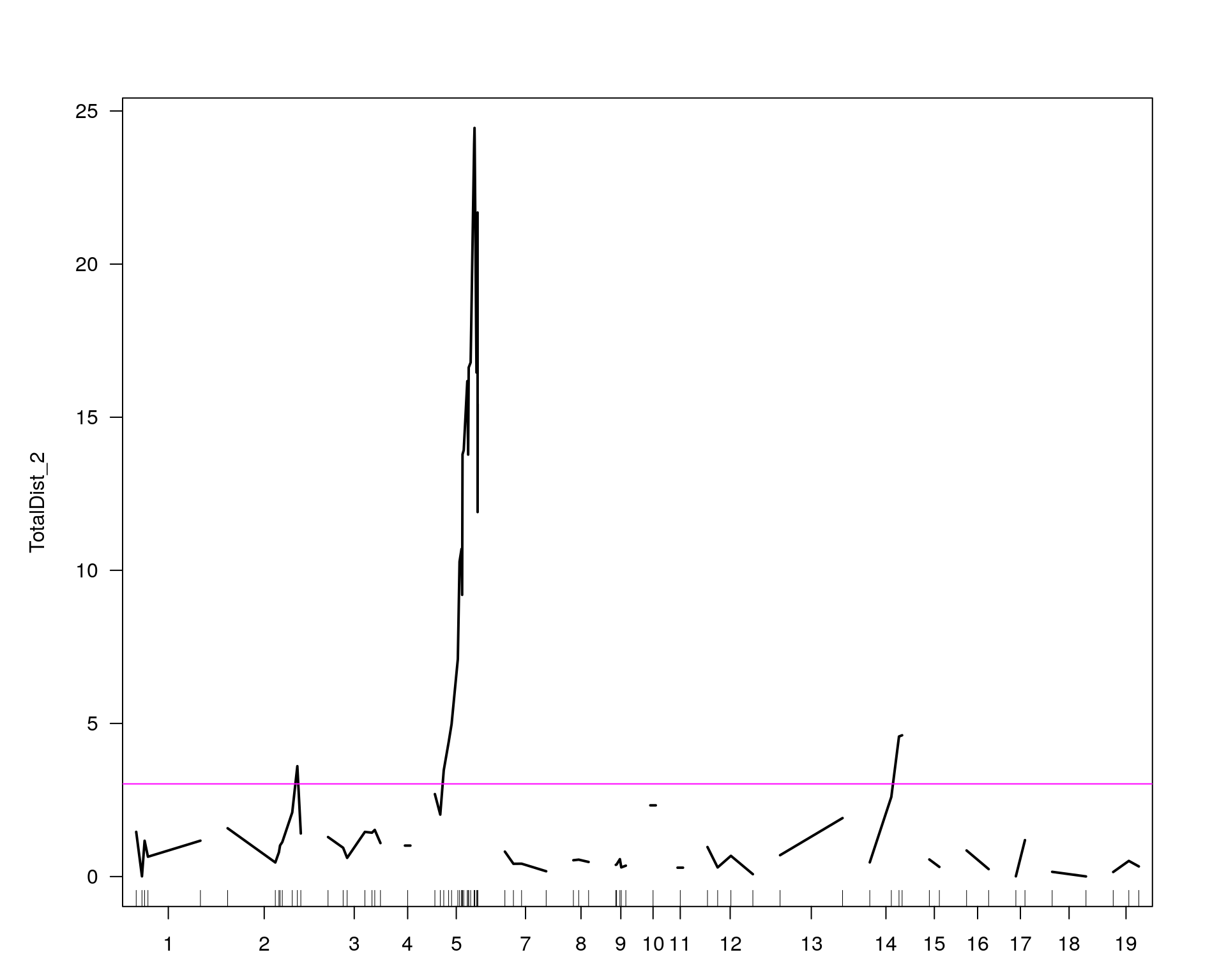
plot(operm[[i]][!is.infinite(operm[[i]])], main=paste(name, colnames(WT144$pheno)[idx[[i]]], sep="-"))
#mrscan_pheno
plot(out.mr[[i]], ylab=colnames(WT144$pheno)[idx[[i]]])
add.threshold(out.mr[[i]], perms = operm[[i]], alpha = 0.05, col="magenta")
#pxg
peak = summary(out.mr[[i]], threshold=summary(operm[[i]], alpha = 0.05)[[1]])
print(peak)
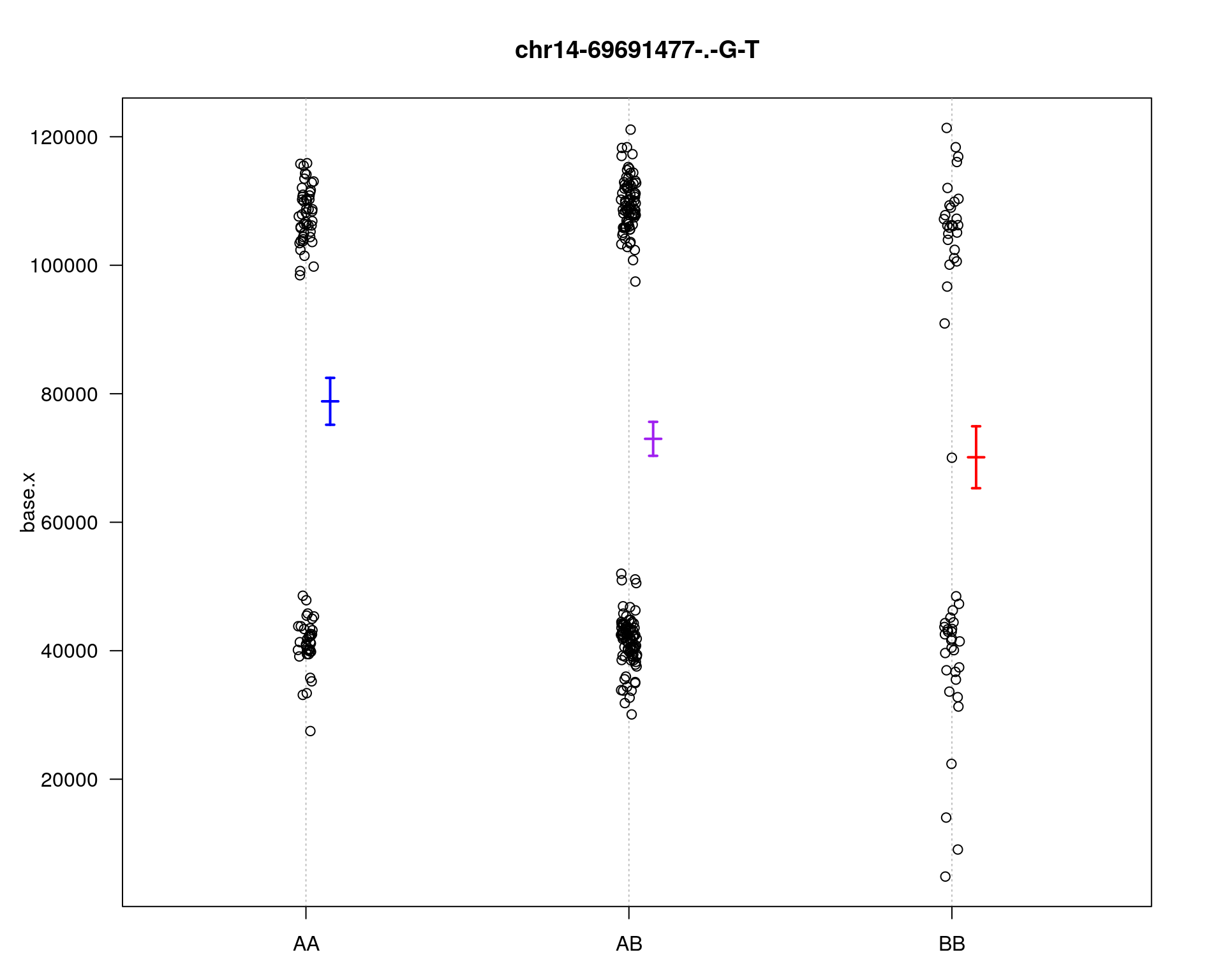
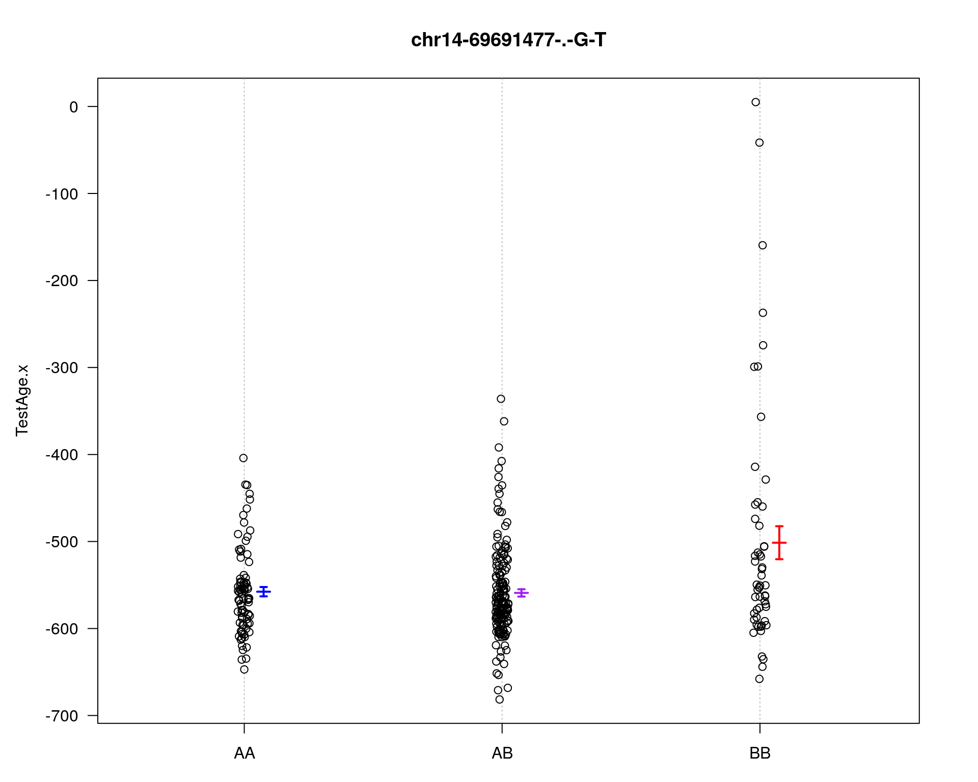
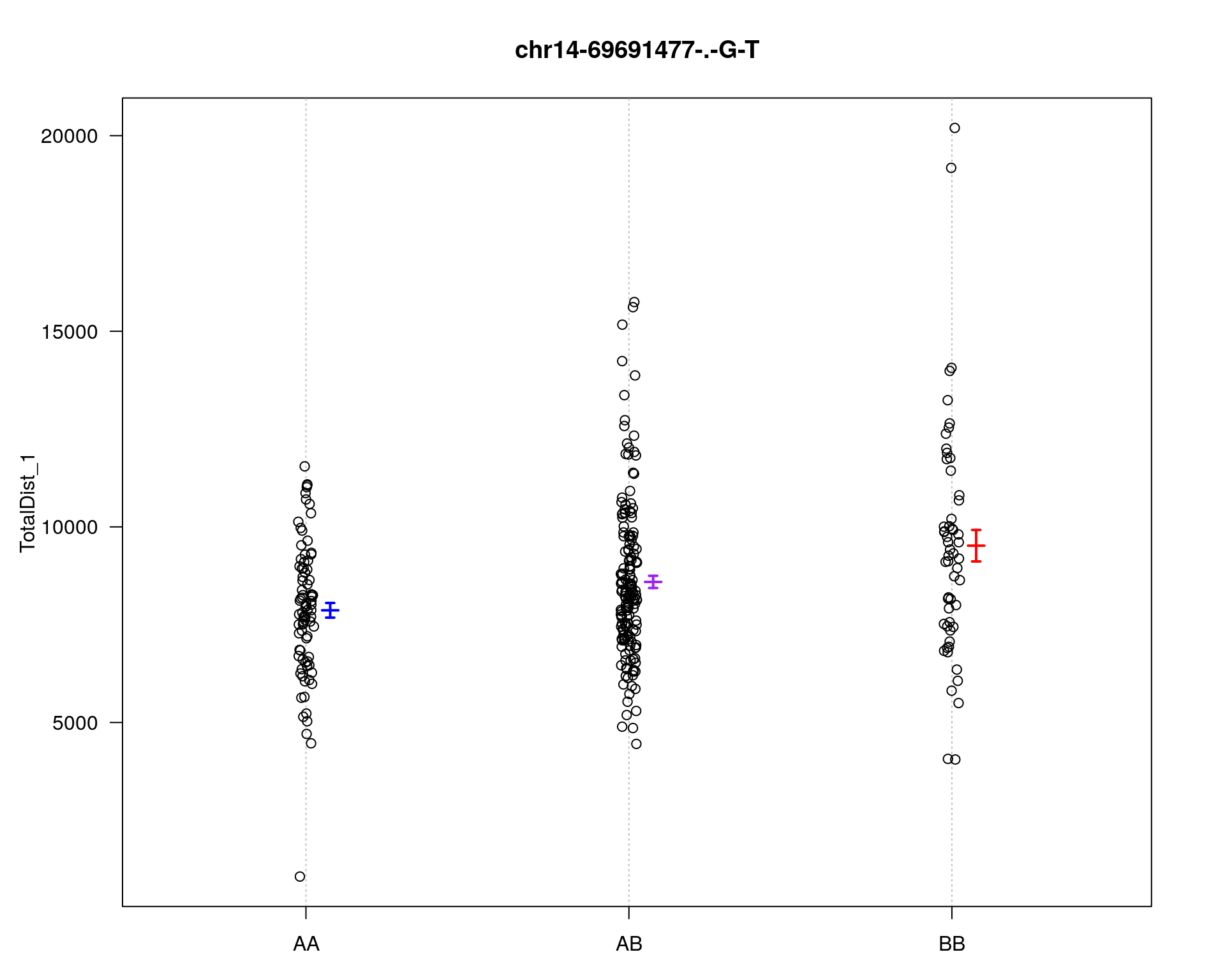
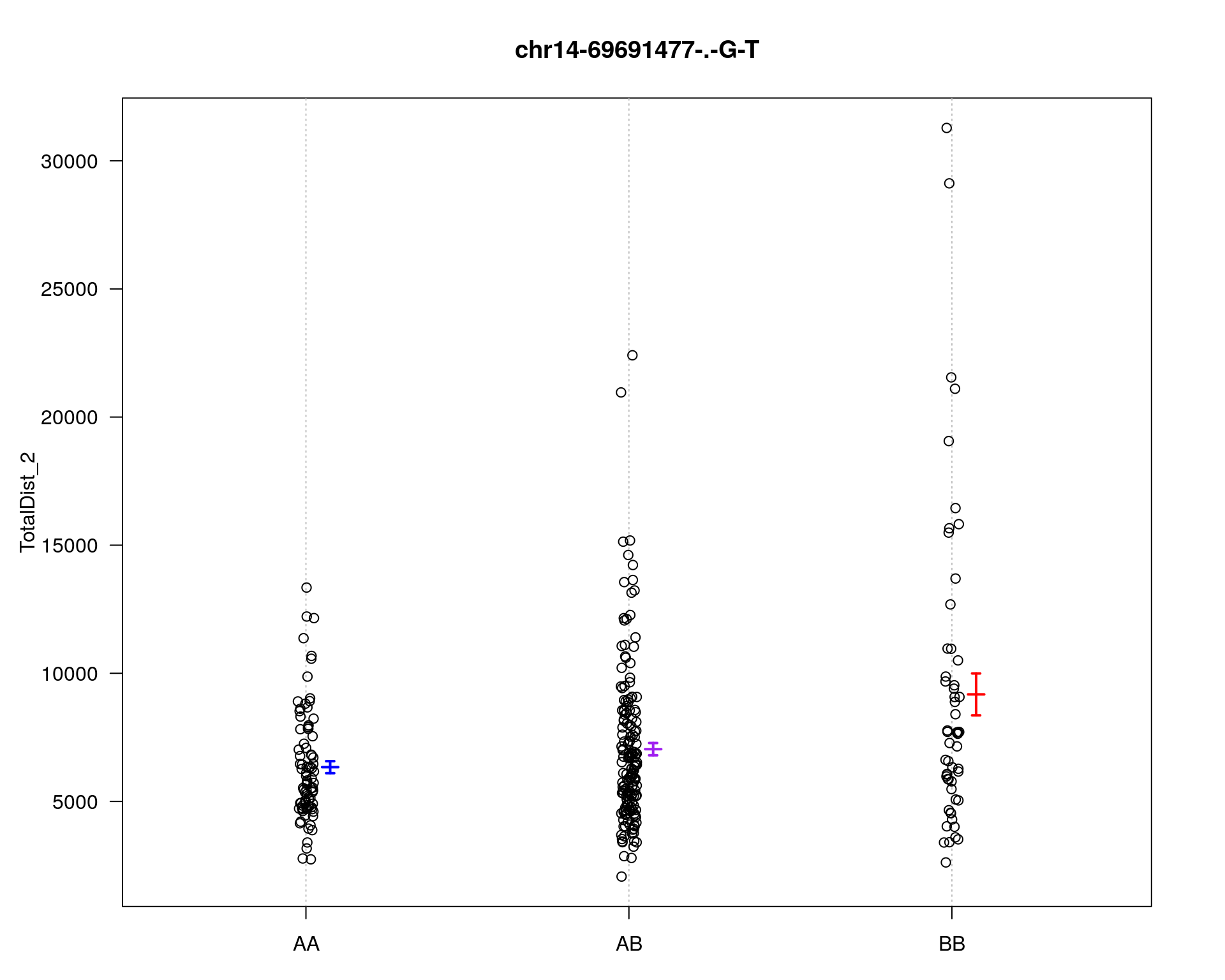
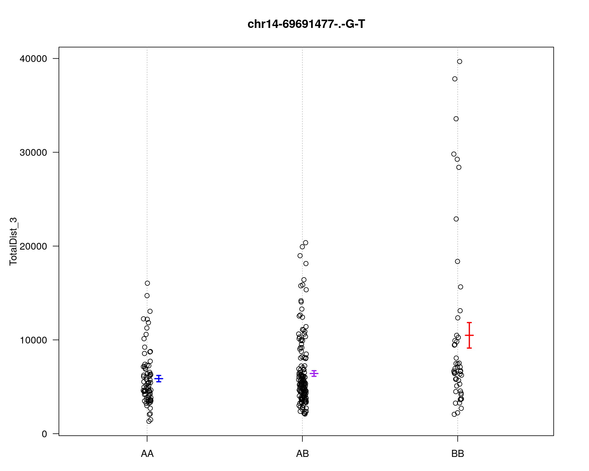
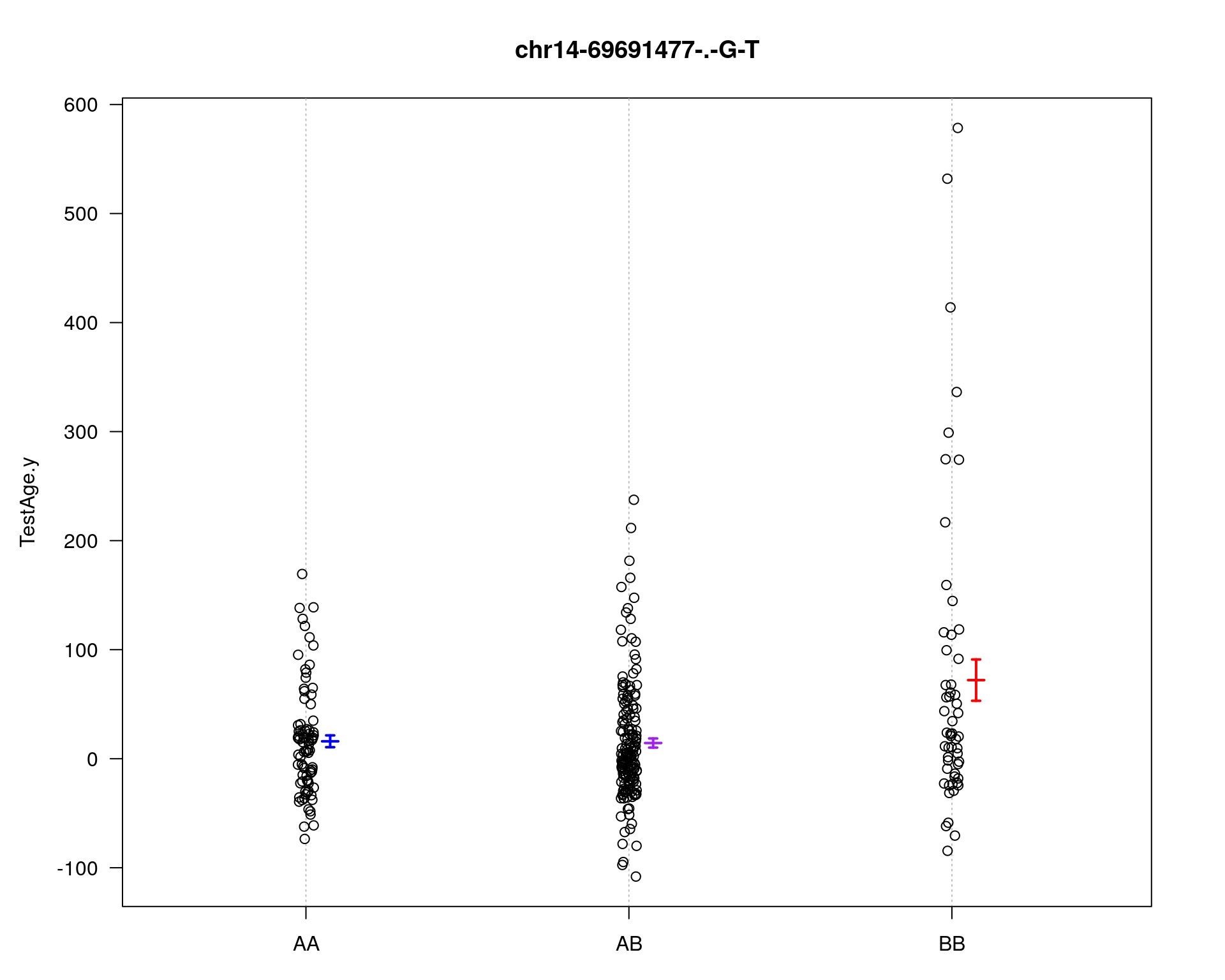
marker = c("chr5-136332619-.-C-A", "chr14-69691477-.-G-T")
for (mar in marker){
par(mar=c(3, 5, 4, 3))
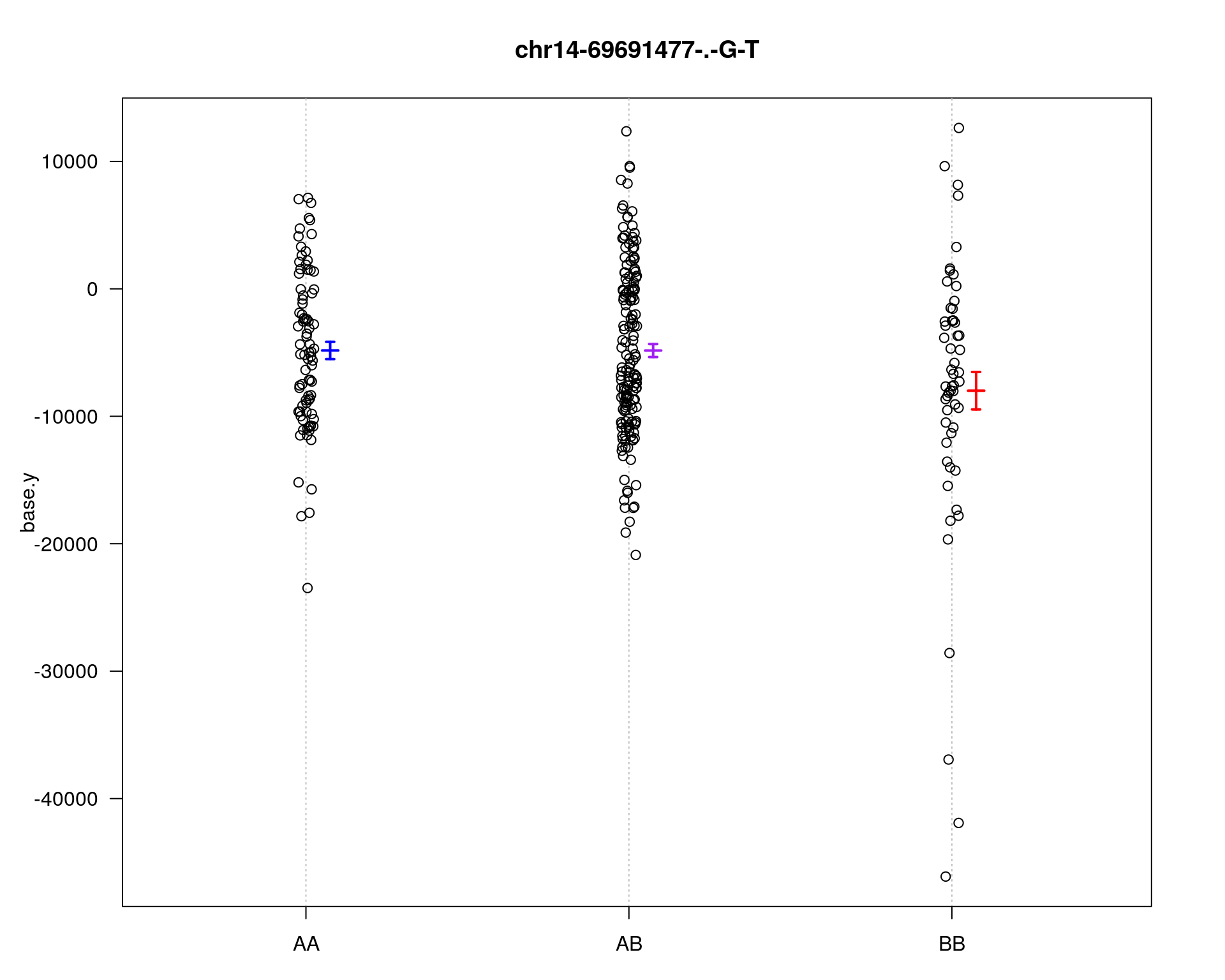
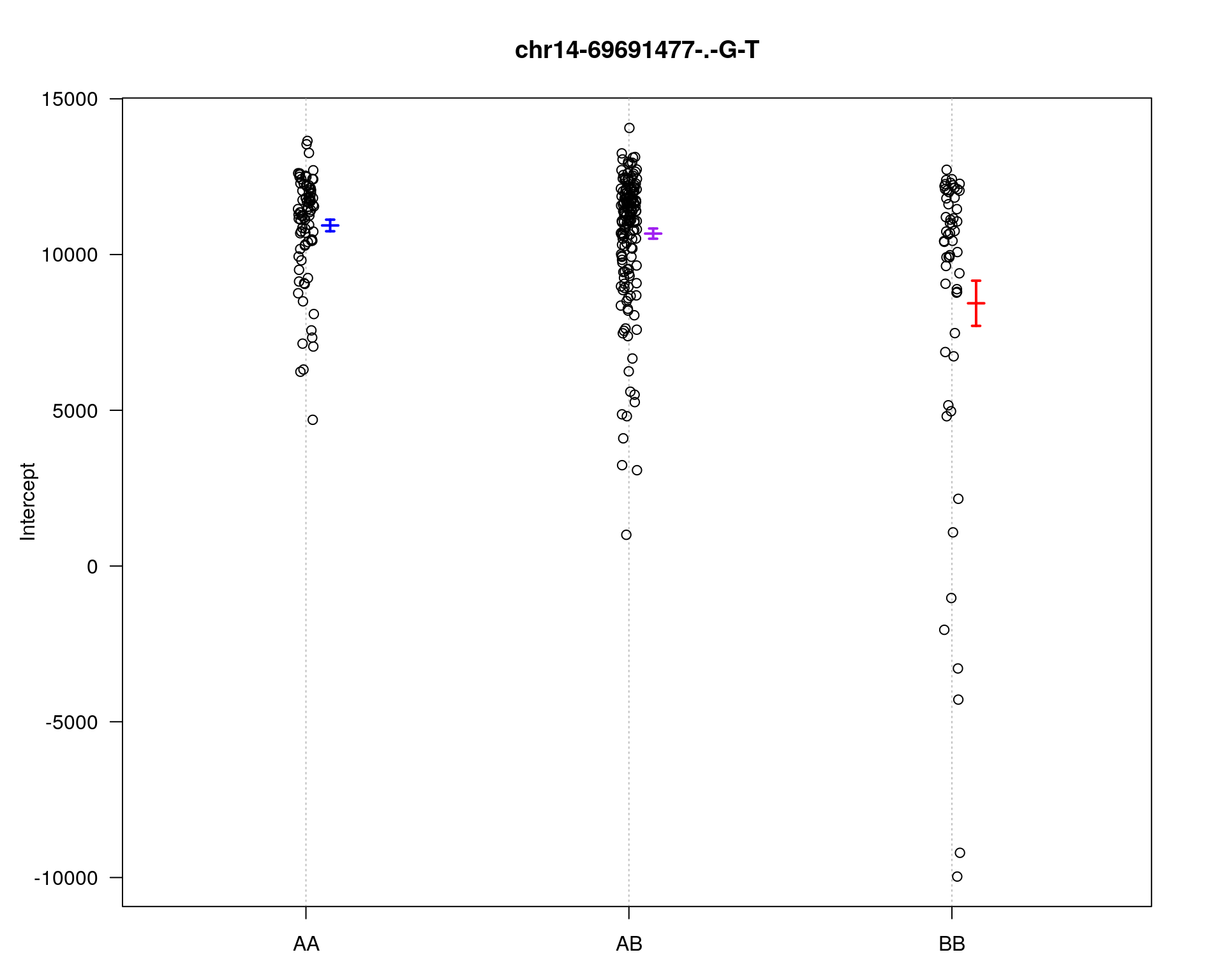
plotPXG(WT144, marker=mar, jitter = 0.25, pheno.col = idx[[i]], infer=F, main=paste(mar),
mgp=c(3.4,1,0))
}
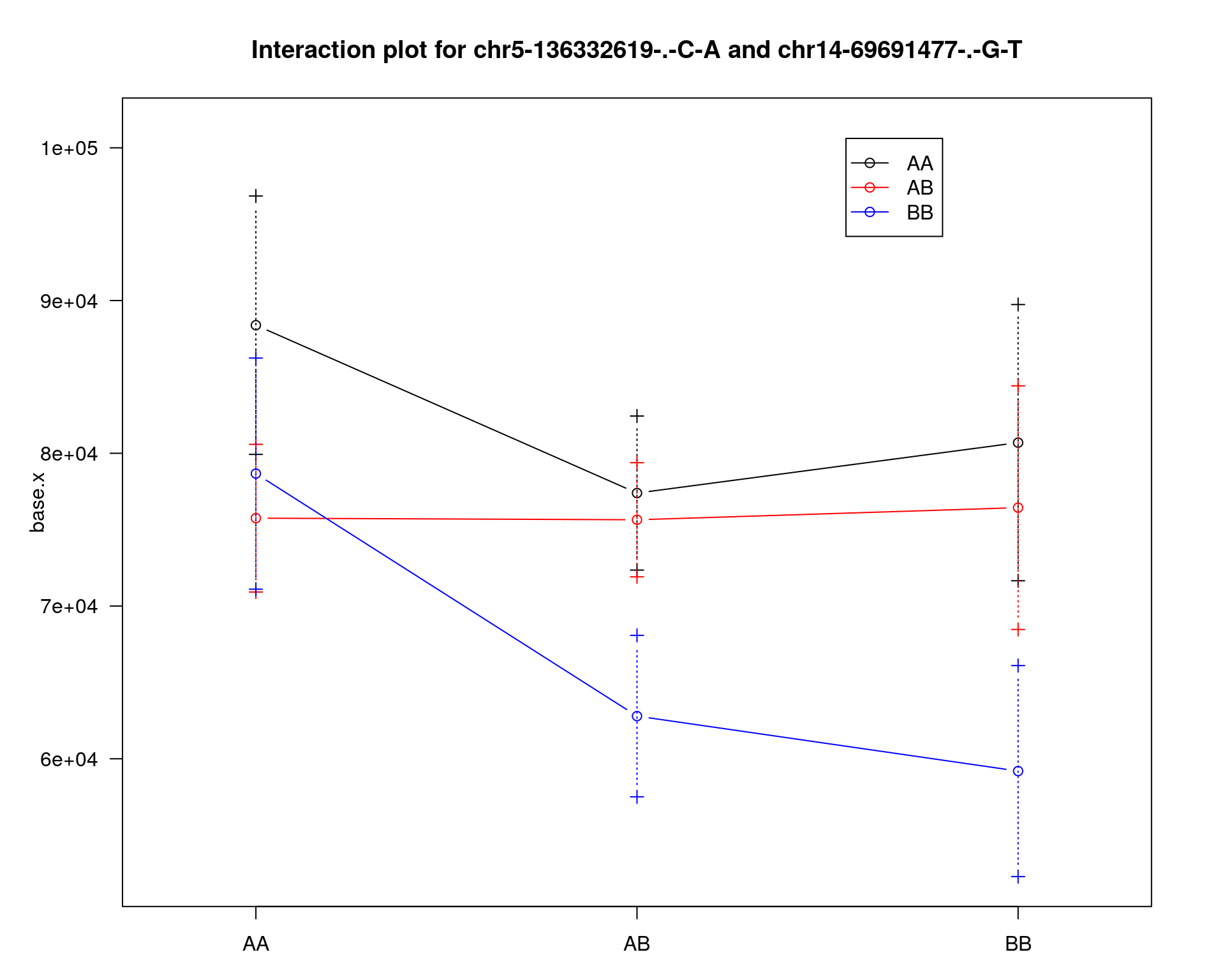
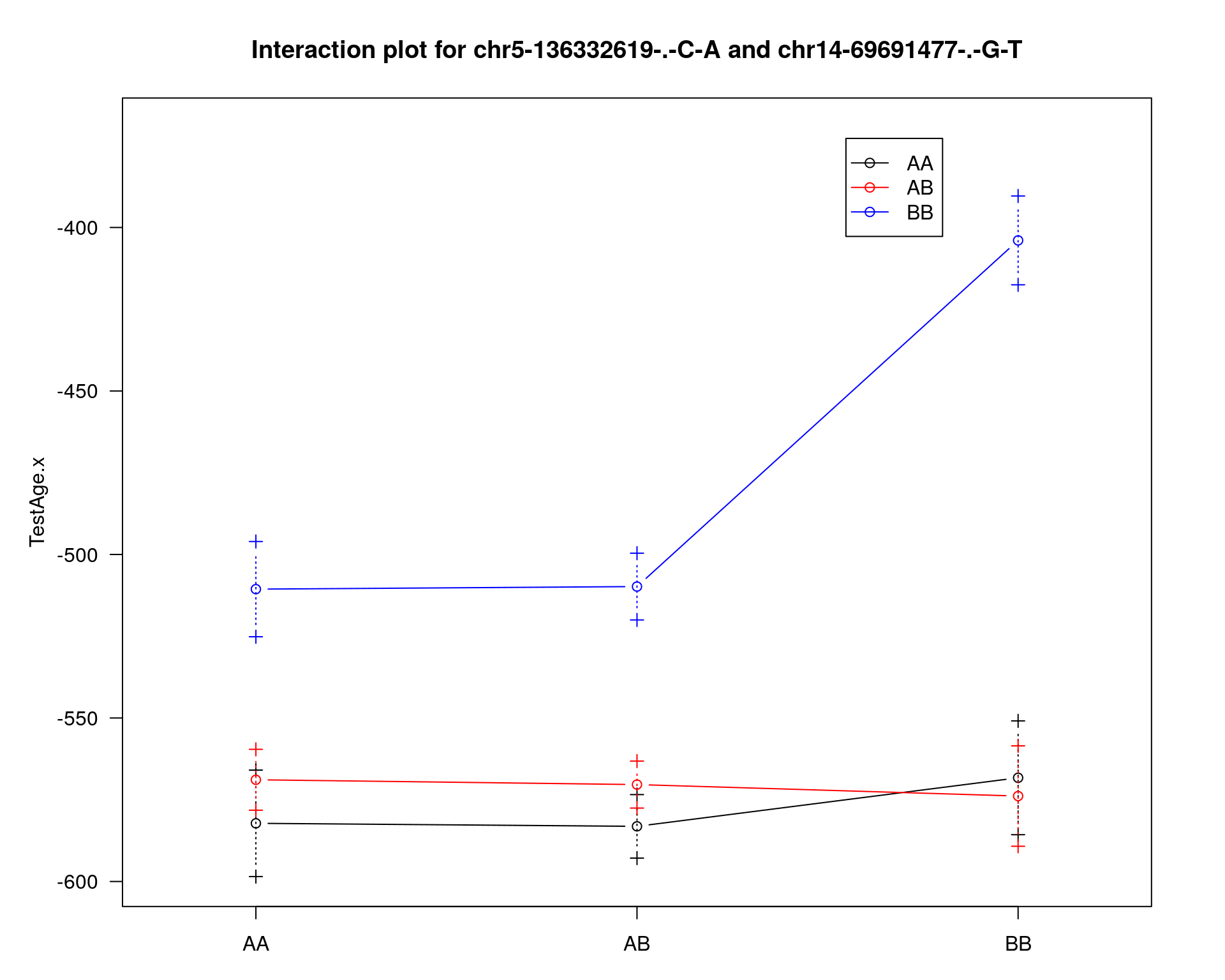
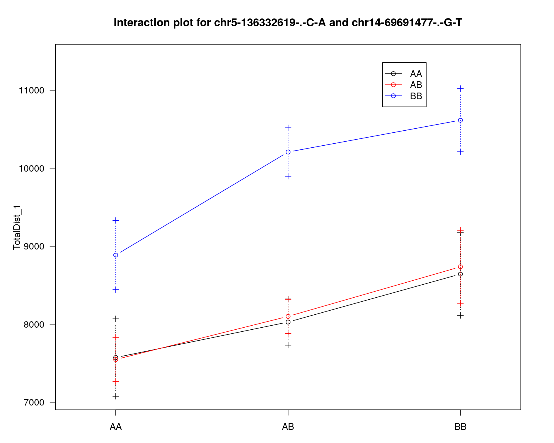
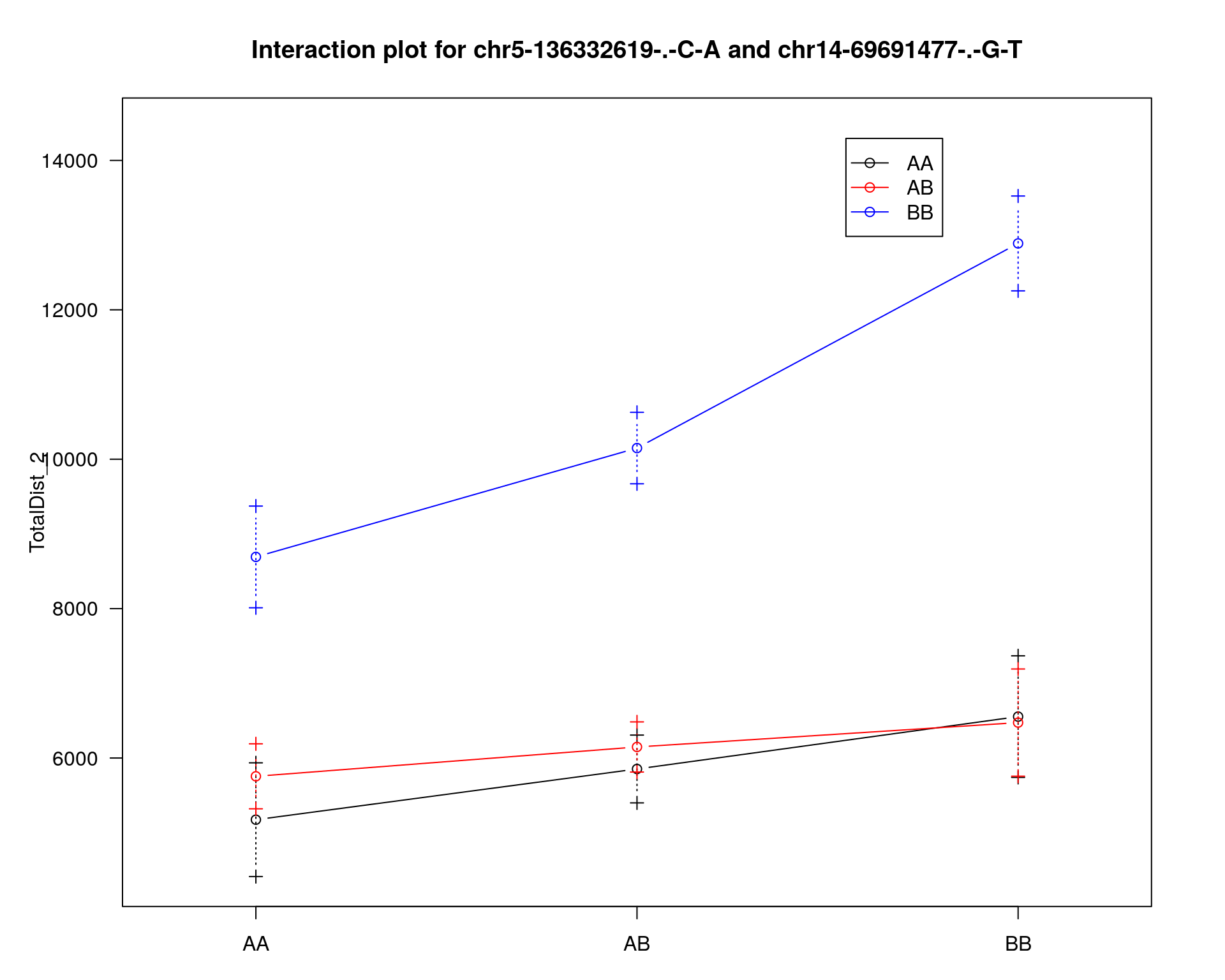
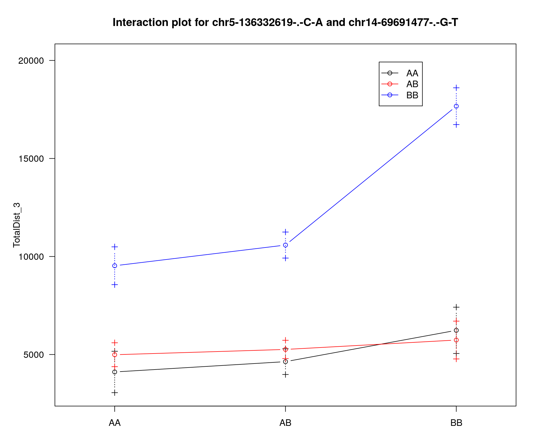
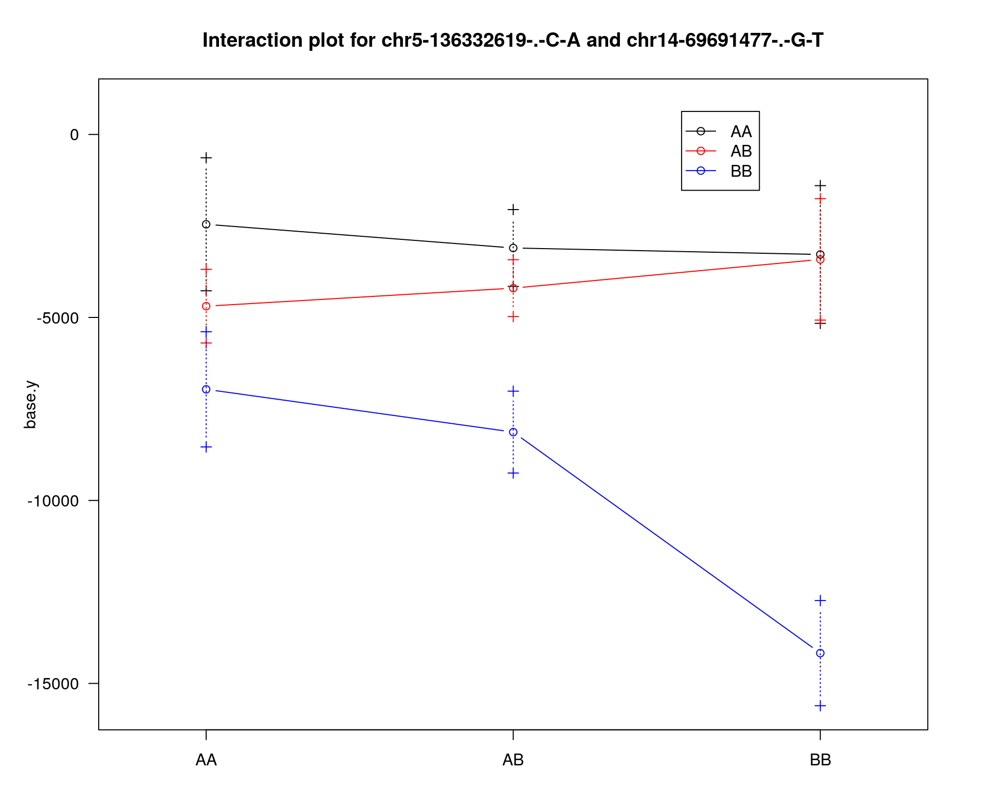
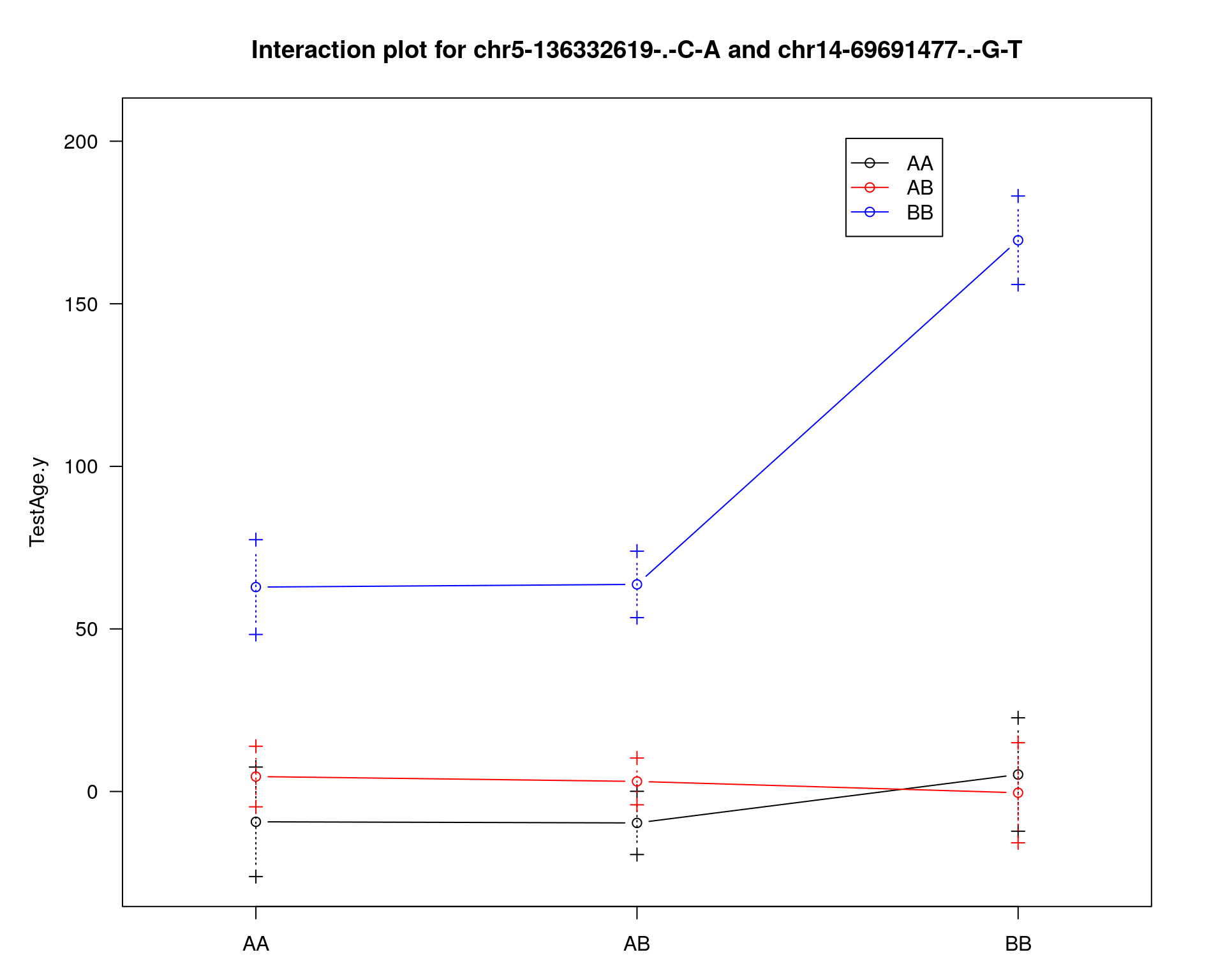
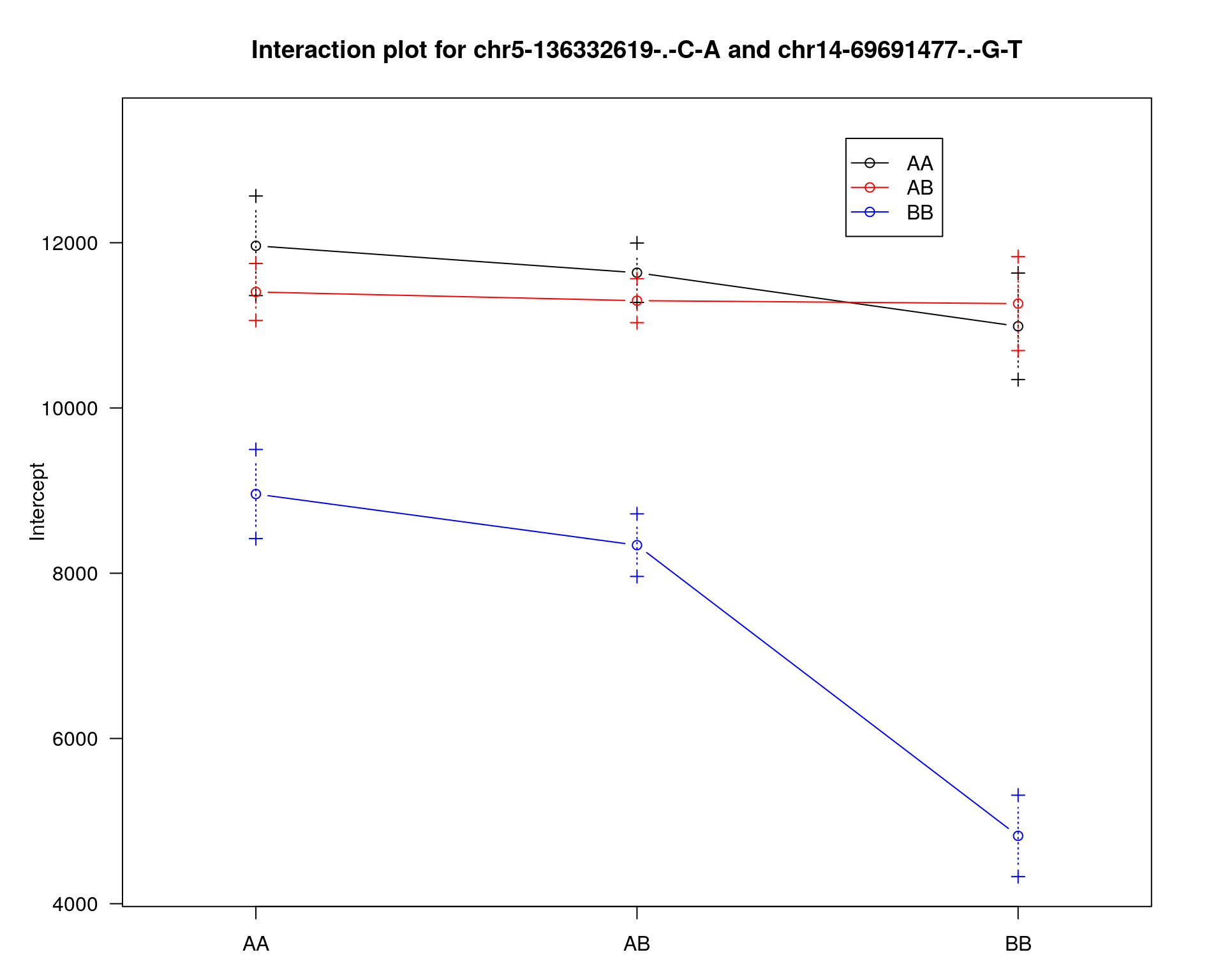
#interaction_effect
effectplot(WT144,
mname1 = marker[[1]],
mname2 = marker[[2]],
pheno.col = idx[[i]], add.legend=T, legend.lab = "")
##Multiple-QTL analyses
# After performing the single- and two-QTL genome scans, it’s best to bring the identified loci together into a joint model, which we then refine and from which we may explore the possibility of further QTL. In this effort, we work with “QTL objects” created by makeqtl(). We fit multiple-QTL models with fitqtl(). A number of additional functions will be introduced below.
#First, we create a QTL object containing the loci on chr 5 and 14.
#chr5-136332619-.-C-A 75.97770
#chr14-69691477-.-G-T 36.07219
WT144 <- sim.geno(WT144, n.draws=64)
qtl <- makeqtl(WT144, chr=c(5,14), pos=c(75.97770, 36.07219), what="draws")
out.fq <- fitqtl(WT144, pheno.col=idx[[i]], qtl=qtl)
print(summary(out.fq))
#We may obtain the estimated effects of the QTL via get.ests=TRUE. We use dropone=FALSE to suppress the drop-one-term analysis.
print(summary(fitqtl(WT144, pheno.col=idx[[i]], qtl=qtl, get.ests=TRUE, dropone=FALSE)))
#To assess the possibility of an interaction between the two QTL, we may fit the model with the interaction, indicated via a model “formula”.
print("To assess the possibility of an interaction between the two QTL")
out.fqi <- fitqtl(WT144, pheno.col=idx[[i]], qtl=qtl, formula=y~Q1+Q2+Q1:Q2)
print(summary(out.fqi))
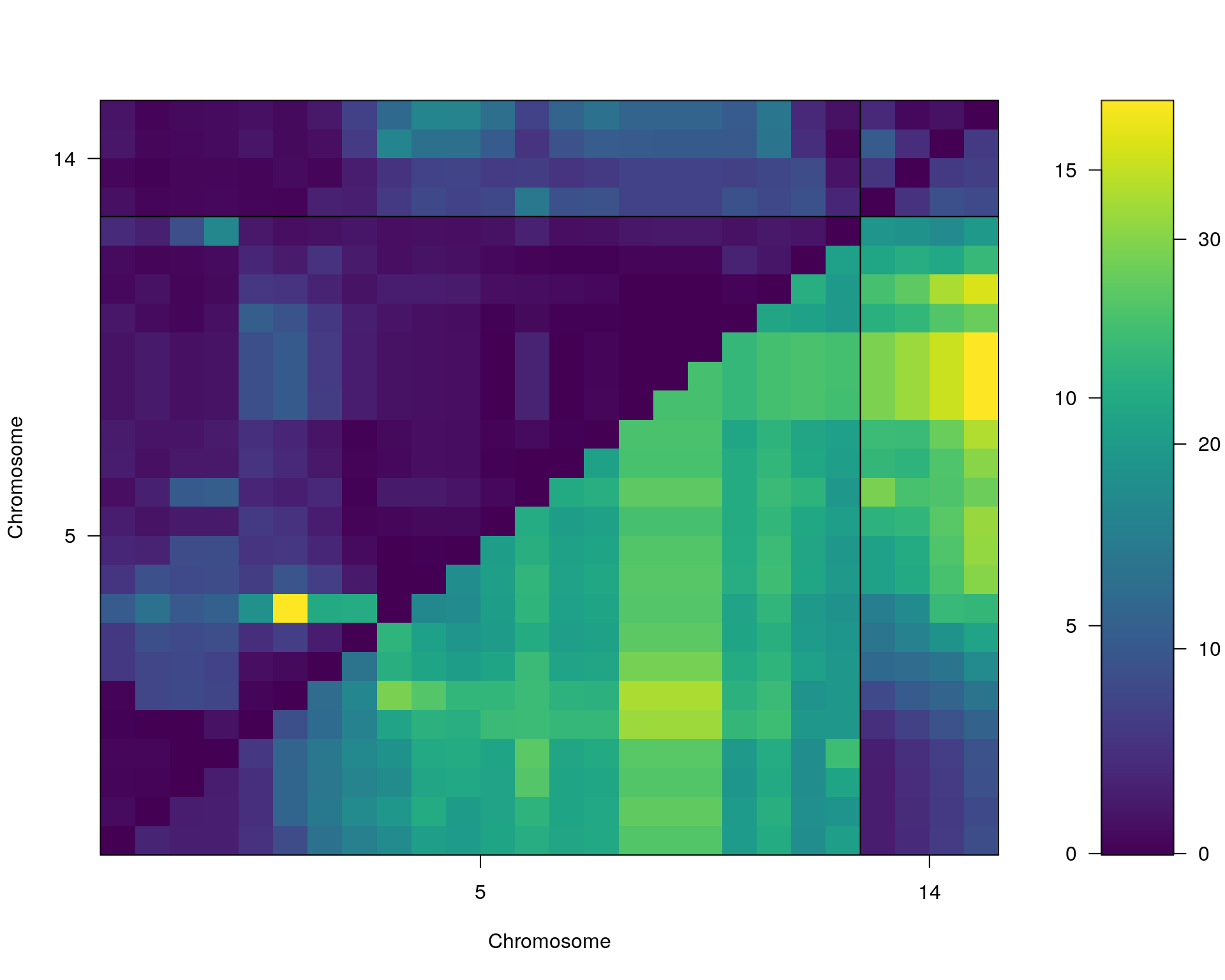
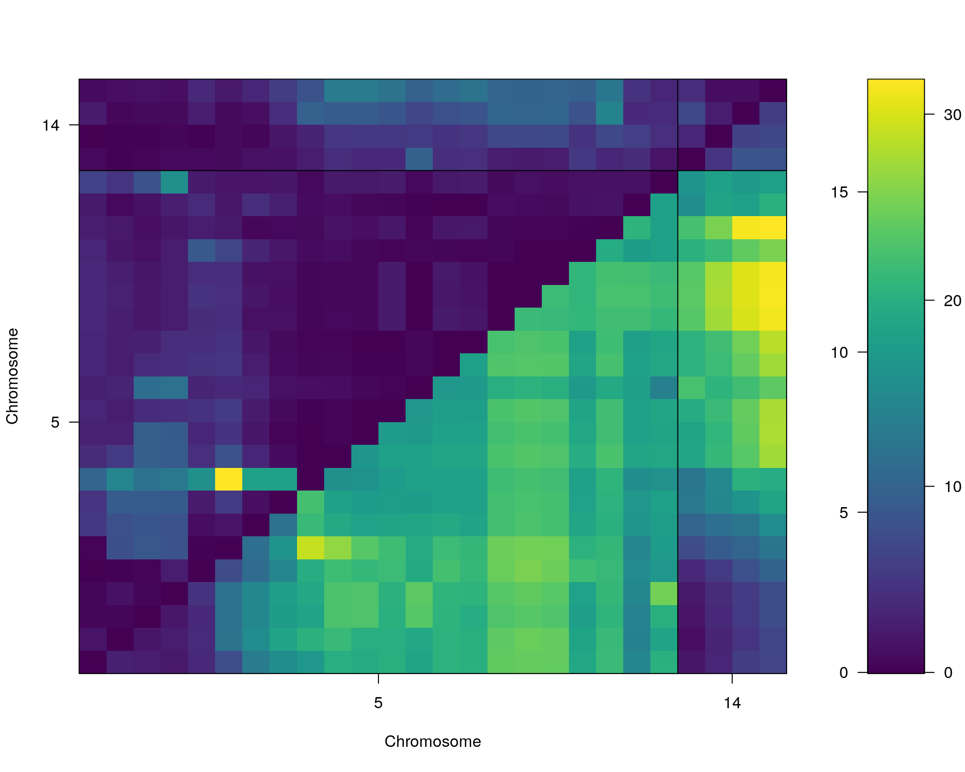
#complete_scan2
plot(st[[i]])
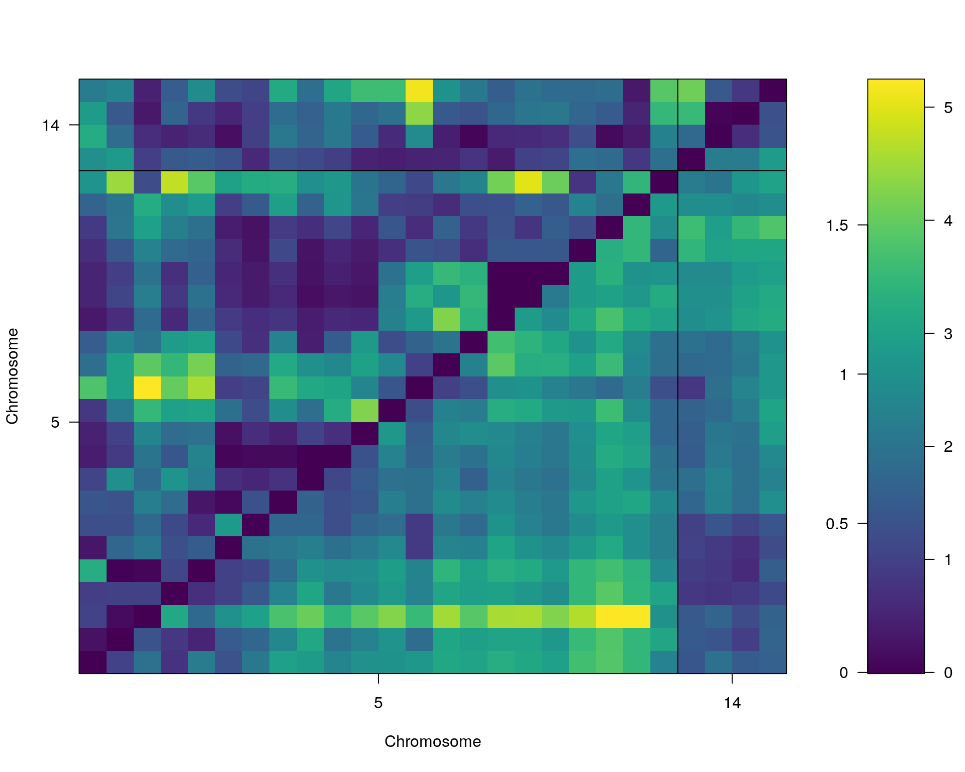
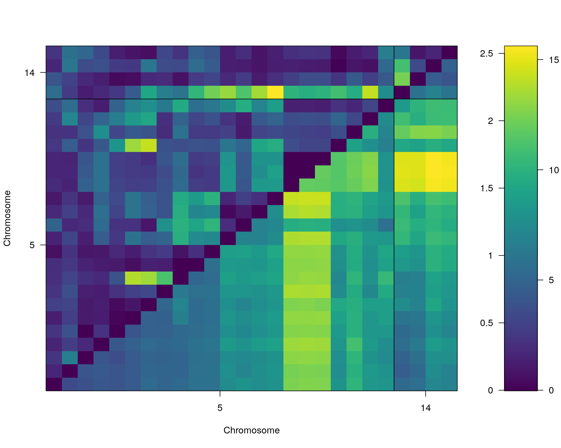
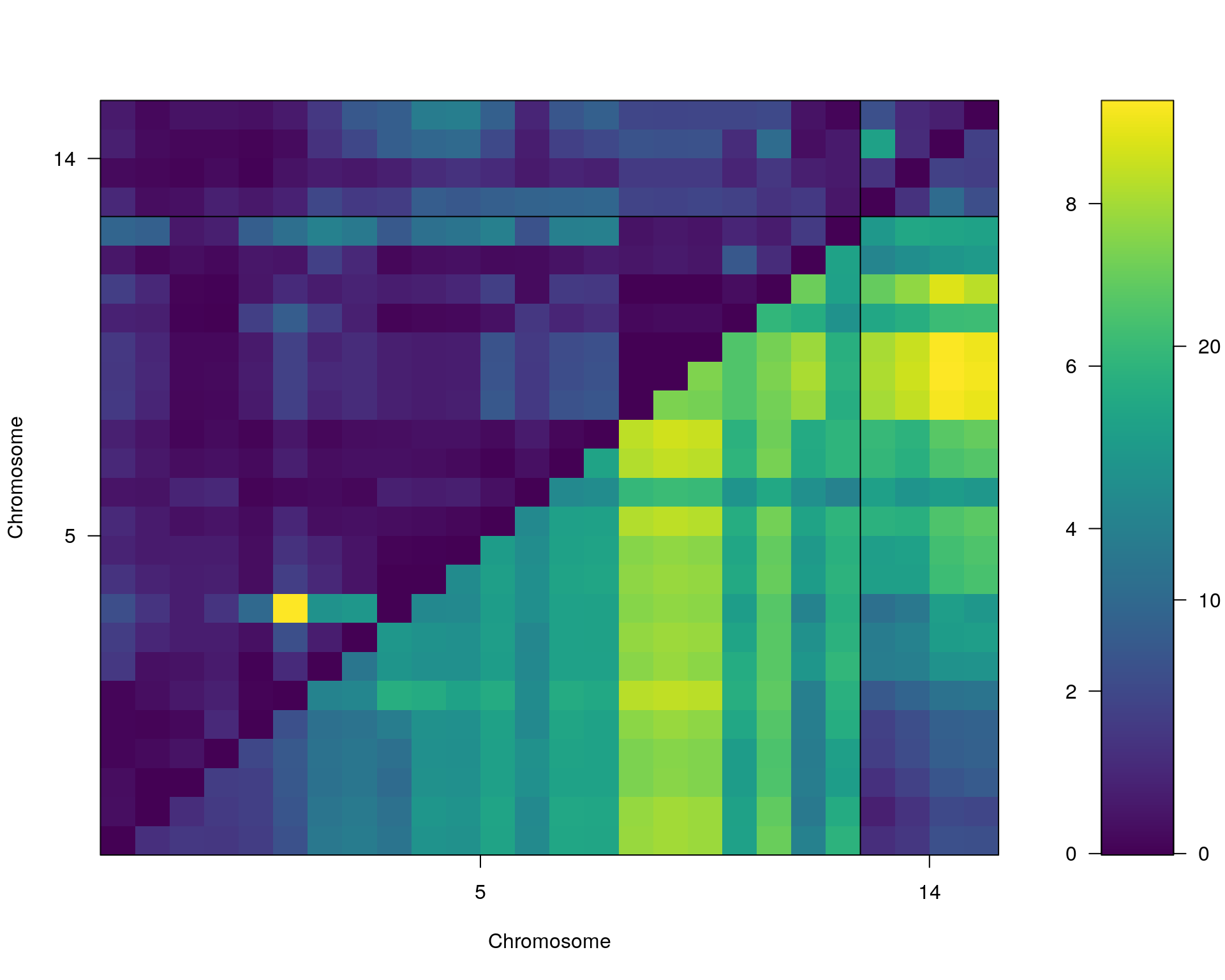
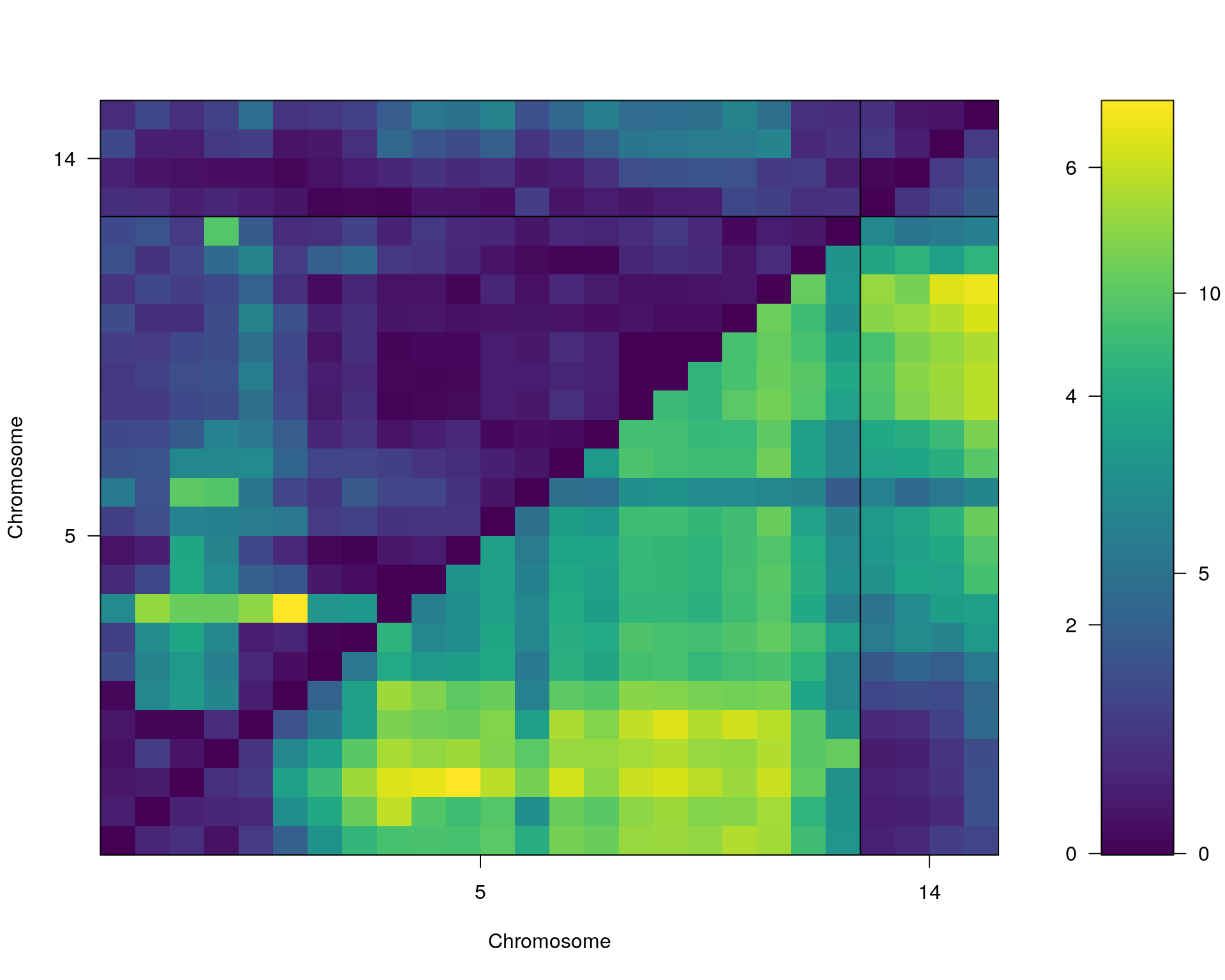
#toptwo_scan2
plot(st[[i]], chr = summary(out.mr[[i]])[order(-summary(out.mr[[i]])$lod), "chr"][1:2])
#dev.off()
}[1] "base.x"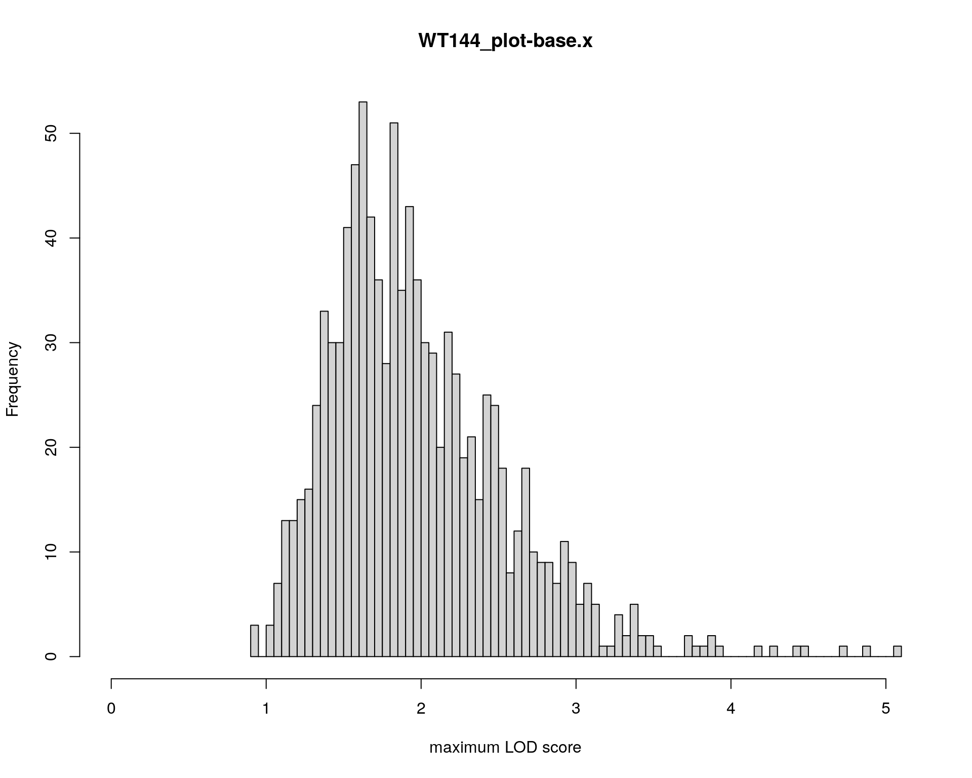
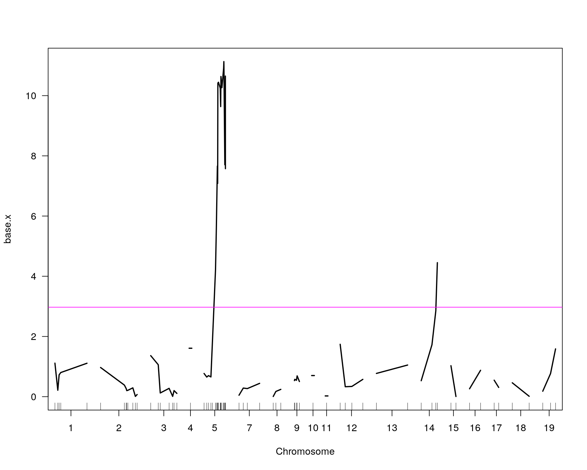
                     chr  pos   lod
chr5-136332619-.-C-A   5 76.0 11.13
chr14-69691477-.-G-T  14 36.1  4.45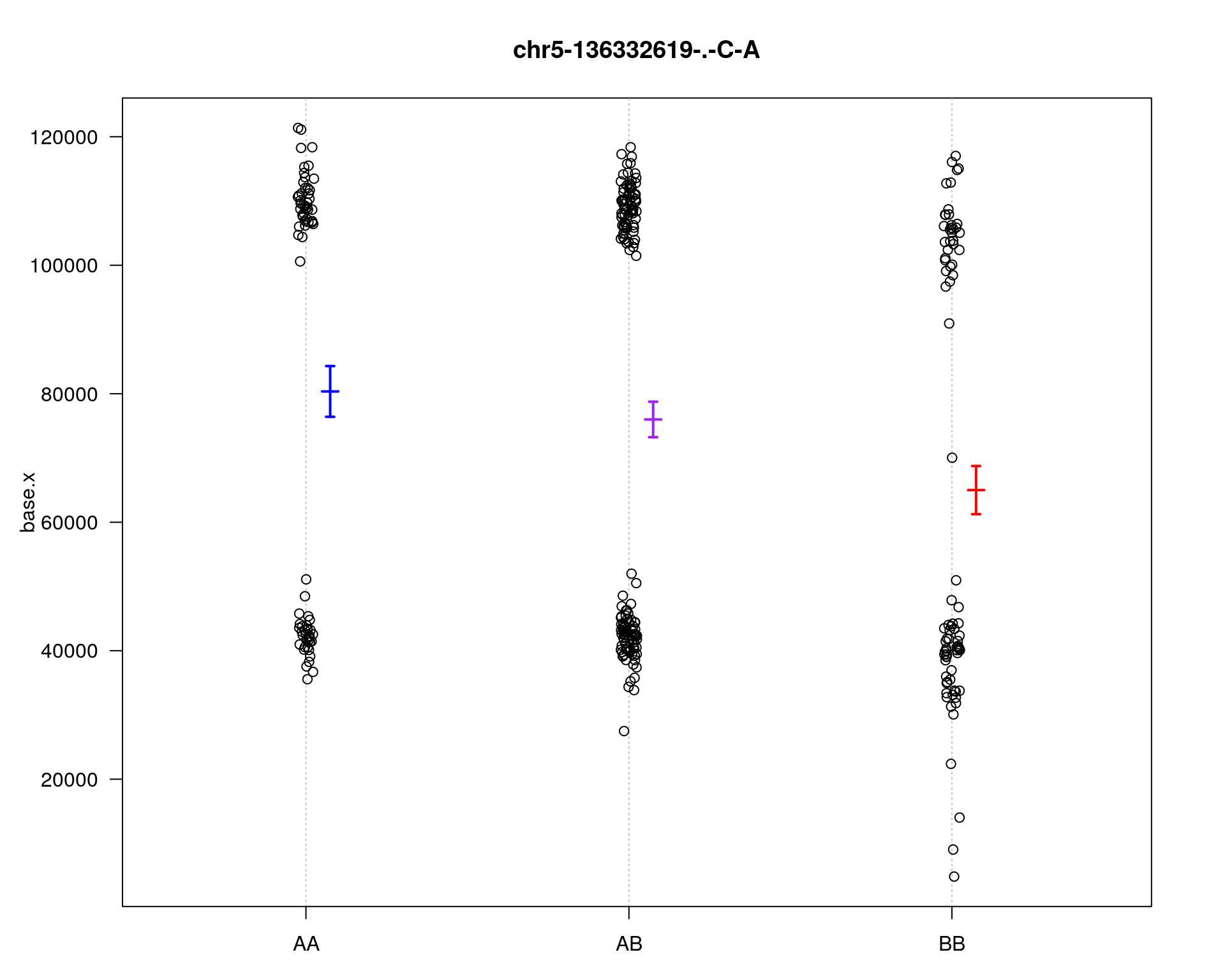
        fitqtl summary

Method: multiple imputation
Model:  normal phenotype
Number of observations : 309

Full model result
----------------------------------
Model formula: y ~ Q1 + Q2

       df           SS         MS      LOD     %var Pvalue(Chi2)  Pvalue(F)
Model   4  12268860063 3067215016 2.288244 3.352781   0.03228092 0.03418567
Error 304 353661975772 1163361762
Total 308 365930835835


Drop one QTL at a time ANOVA table:
----------------------------------
        df Type III SS    LOD   %var F value Pvalue(Chi2) Pvalue(F)
5@76.0   2   9.277e+09 1.7374 2.5352   3.987        0.018    0.0195 *
14@36.1  2   2.548e+09 0.4817 0.6963   1.095        0.330    0.3358
---
Signif. codes:  0 '***' 0.001 '**' 0.01 '*' 0.05 '.' 0.1 ' ' 1


        fitqtl summary

Method: multiple imputation
Model:  normal phenotype
Number of observations : 309

Full model result
----------------------------------
Model formula: y ~ Q1 + Q2

       df           SS         MS      LOD     %var Pvalue(Chi2)  Pvalue(F)
Model   4  12268860063 3067215016 2.288244 3.352781   0.03228092 0.03418567
Error 304 353661975772 1163361762
Total 308 365930835835


Estimated effects:
-----------------
            est    SE      t
Intercept 74118  1978 37.469
5@76.0a   -7480  2718 -2.752
5@76.0d    2152  3946  0.545
14@36.1a  -3590  2982 -1.204
14@36.1d  -2592  3963 -0.654

[1] "To assess the possibility of an interaction between the two QTL"

        fitqtl summary

Method: multiple imputation
Model:  normal phenotype
Number of observations : 309

Full model result
----------------------------------
Model formula: y ~ Q1 + Q2 + Q1:Q2

       df           SS         MS      LOD     %var Pvalue(Chi2)  Pvalue(F)
Model   8  15919207151 1989900894 2.984405 4.350332   0.08869552 0.09648892
Error 300 350011628684 1166705429
Total 308 365930835835


Drop one QTL at a time ANOVA table:
----------------------------------
               df Type III SS    LOD   %var F value Pvalue(Chi2) Pvalue(F)
5@76.0          6   1.293e+10 2.4336 3.5328  1.8467        0.082    0.0898 .
14@36.1         6   6.198e+09 1.1778 1.6938  0.8854        0.491    0.5058
5@76.0:14@36.1  4   3.650e+09 0.6962 0.9976  0.7822        0.524    0.5375
---
Signif. codes:  0 '***' 0.001 '**' 0.01 '*' 0.05 '.' 0.1 ' ' 1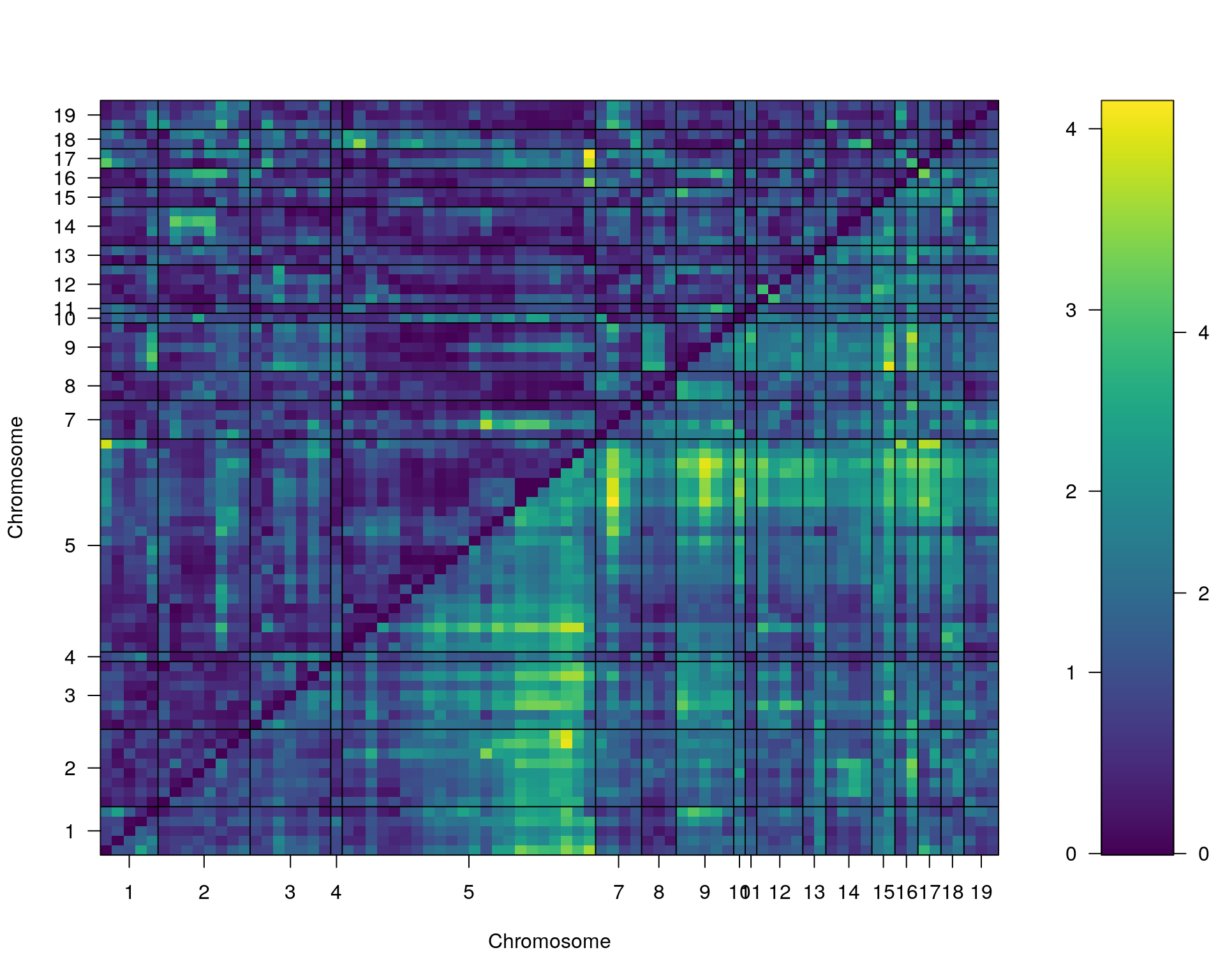
[1] "TestAge.x"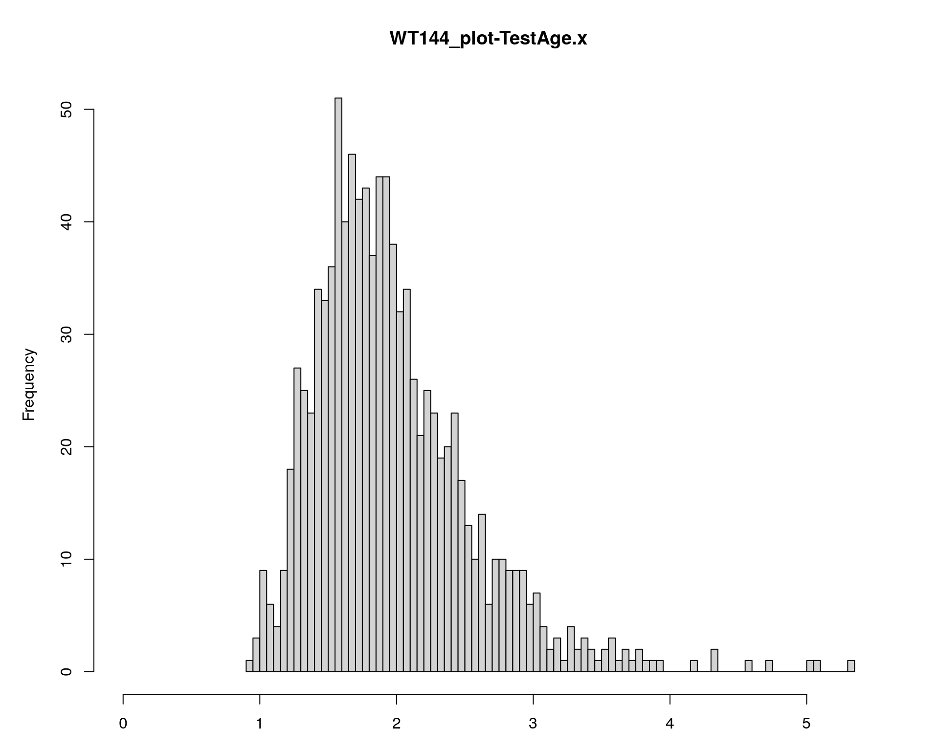
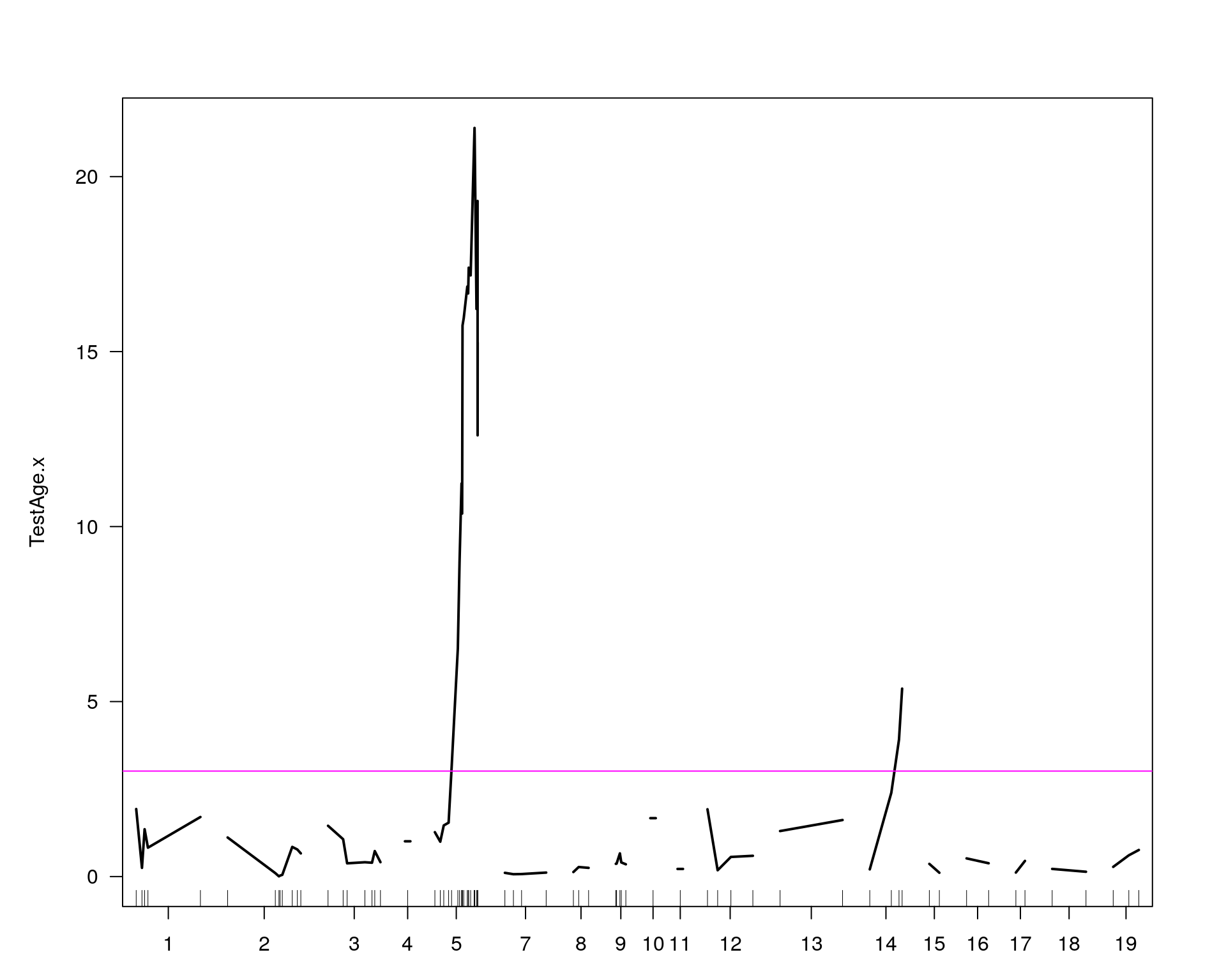
                     chr  pos   lod
chr5-136332619-.-C-A   5 76.0 21.39
chr14-69691477-.-G-T  14 36.1  5.37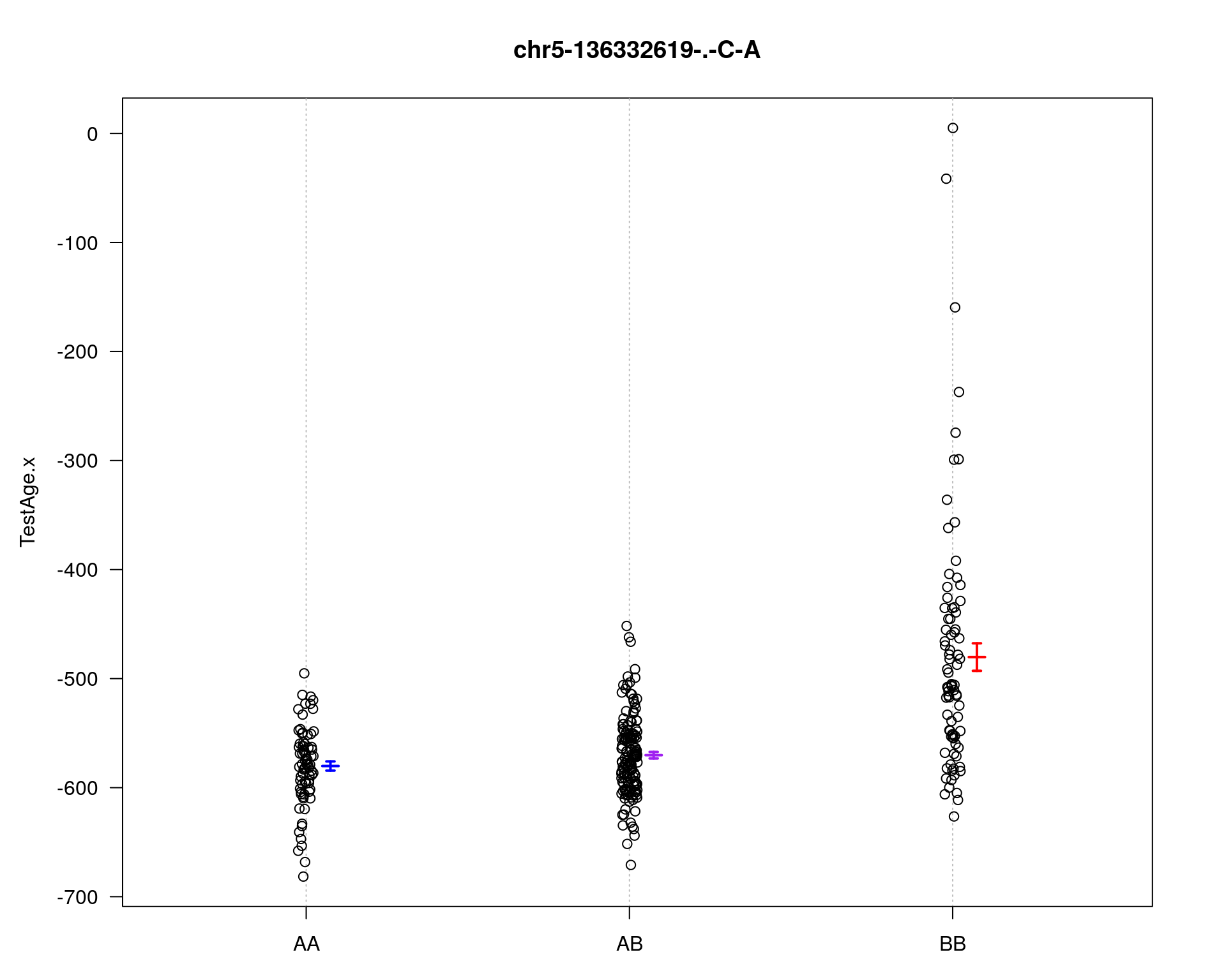
        fitqtl summary

Method: multiple imputation
Model:  normal phenotype
Number of observations : 308

Full model result
----------------------------------
Model formula: y ~ Q1 + Q2

       df        SS         MS      LOD     %var Pvalue(Chi2) Pvalue(F)
Model   4  608423.7 152105.932 25.57375 31.77608            0         0
Error 303 1306298.9   4311.218
Total 307 1914722.7


Drop one QTL at a time ANOVA table:
----------------------------------
        df Type III SS   LOD   %var F value Pvalue(Chi2) Pvalue(F)
5@76.0   2      460384 20.19 24.044   53.39            0   < 2e-16 ***
14@36.1  2       80099  3.98  4.183    9.29            0  0.000121 ***
---
Signif. codes:  0 '***' 0.001 '**' 0.01 '*' 0.05 '.' 0.1 ' ' 1


        fitqtl summary

Method: multiple imputation
Model:  normal phenotype
Number of observations : 308

Full model result
----------------------------------
Model formula: y ~ Q1 + Q2

       df        SS         MS      LOD     %var Pvalue(Chi2) Pvalue(F)
Model   4  608423.7 152105.932 25.57375 31.77608            0         0
Error 303 1306298.9   4311.218
Total 307 1914722.7


Estimated effects:
-----------------
               est       SE        t
Intercept -547.265    3.819 -143.309
5@76.0a     47.707    5.244    9.097
5@76.0d    -35.126    7.593   -4.626
14@36.1a    20.989    5.766    3.640
14@36.1d   -22.016    7.650   -2.878

[1] "To assess the possibility of an interaction between the two QTL"

        fitqtl summary

Method: multiple imputation
Model:  normal phenotype
Number of observations : 308

Full model result
----------------------------------
Model formula: y ~ Q1 + Q2 + Q1:Q2

       df        SS        MS      LOD     %var Pvalue(Chi2) Pvalue(F)
Model   8  719152.1 89894.014 31.49772 37.55907            0         0
Error 299 1195570.6  3998.564
Total 307 1914722.7


Drop one QTL at a time ANOVA table:
----------------------------------
               df Type III SS    LOD   %var F value Pvalue(Chi2) Pvalue(F)
5@76.0          6      571112 26.116 29.827  23.805            0   < 2e-16 ***
14@36.1         6      190827  9.904  9.966   7.954            0  5.70e-08 ***
5@76.0:14@36.1  4      110728  5.924  5.783   6.923            0  2.43e-05 ***
---
Signif. codes:  0 '***' 0.001 '**' 0.01 '*' 0.05 '.' 0.1 ' ' 1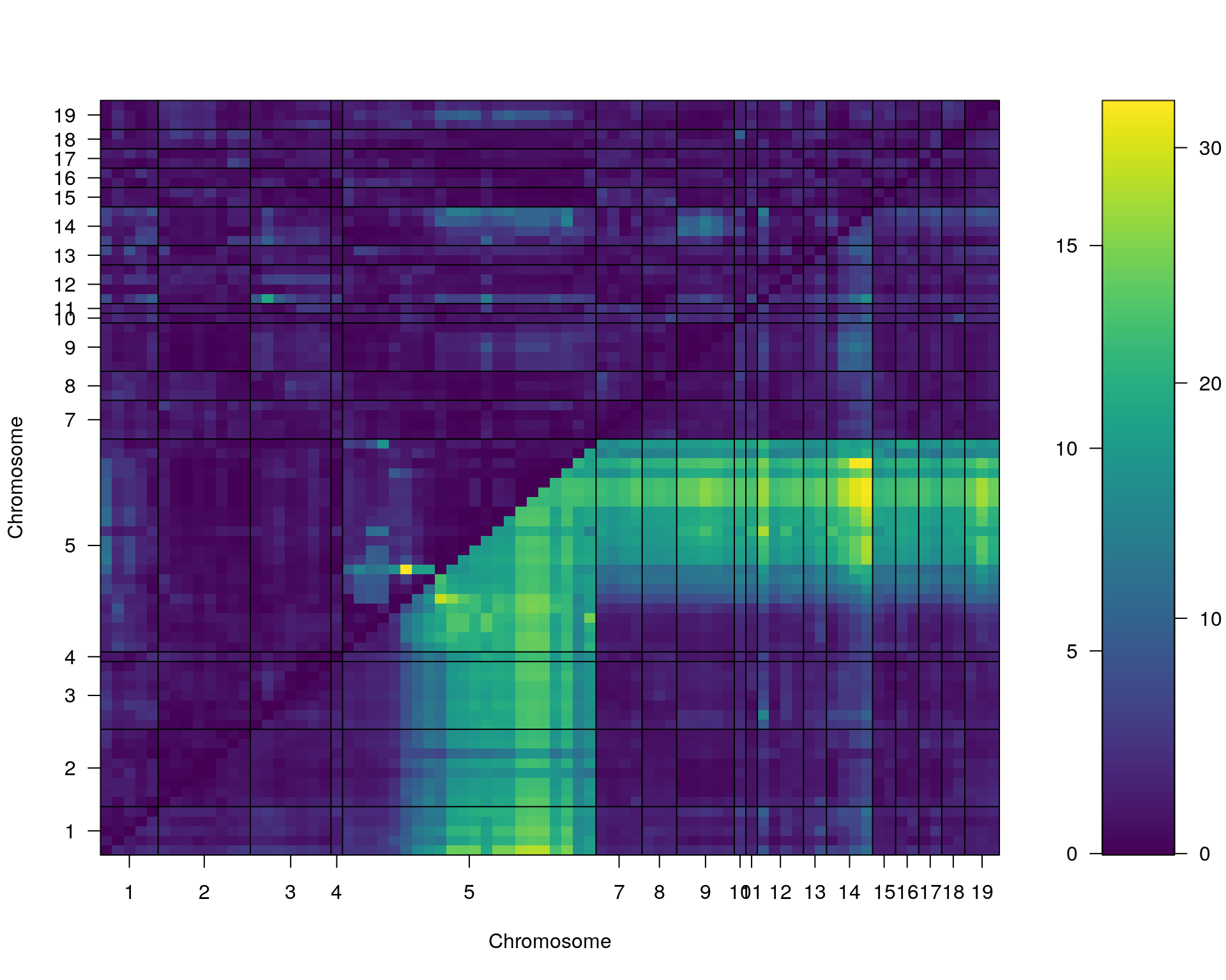

[1] "TotalDist_1"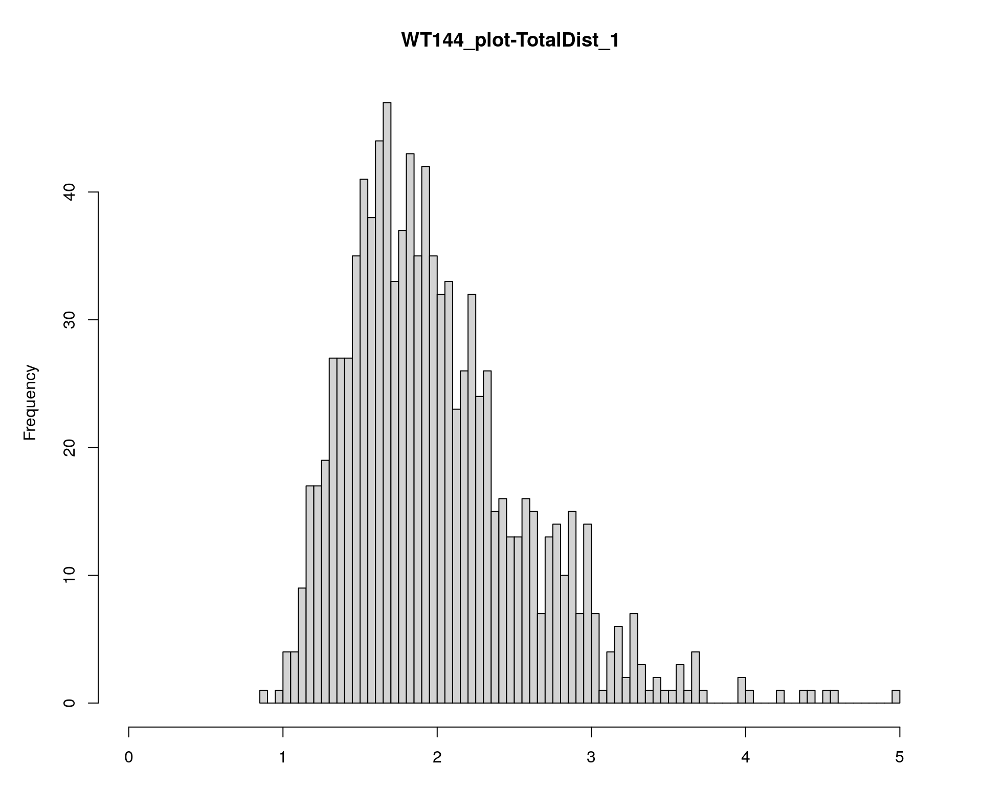
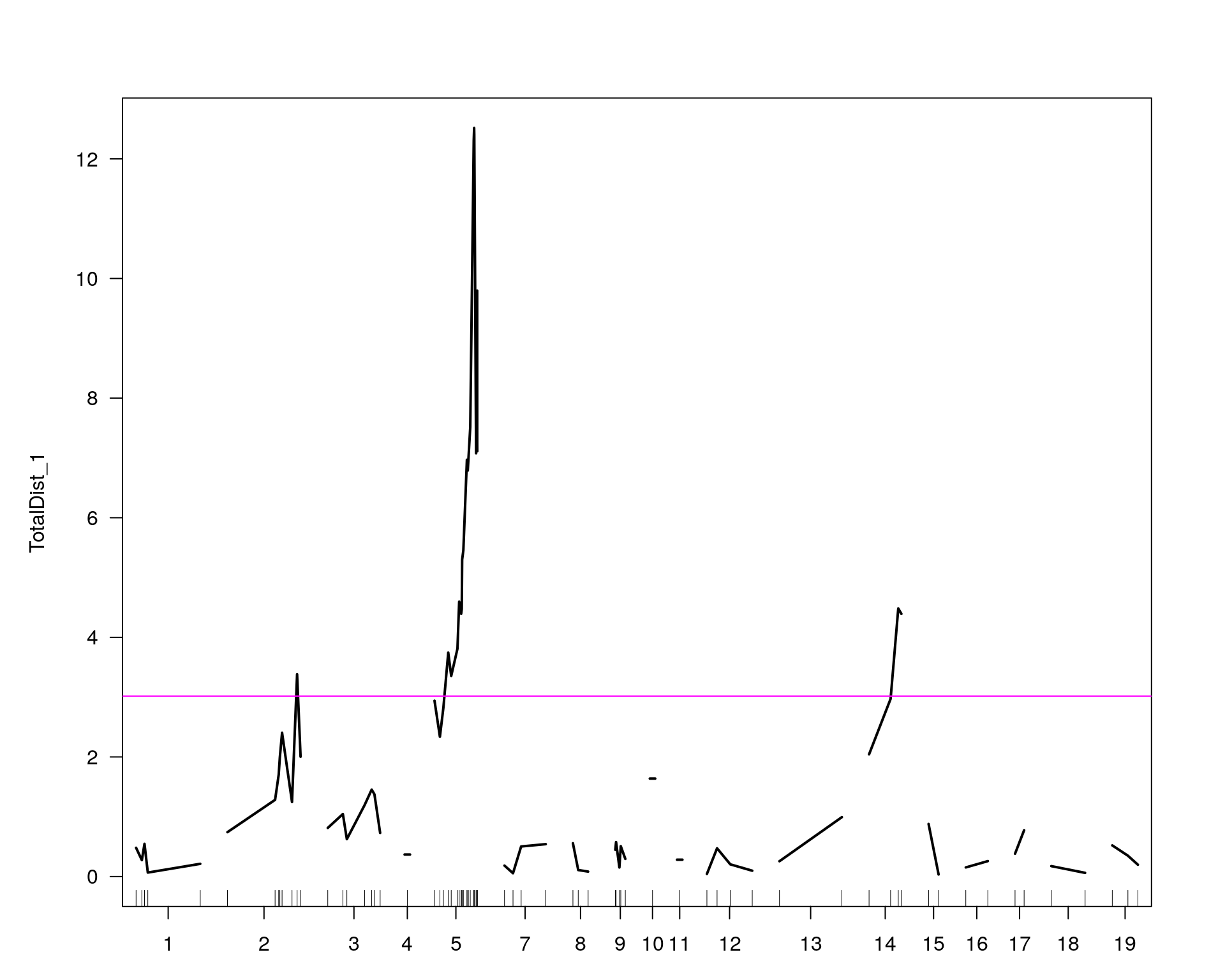
                     chr  pos   lod
chr2-137498061-.-T-A   2 67.9  3.38
chr5-136332619-.-C-A   5 76.0 12.52
chr14-62407765-.-T-A  14 33.2  4.48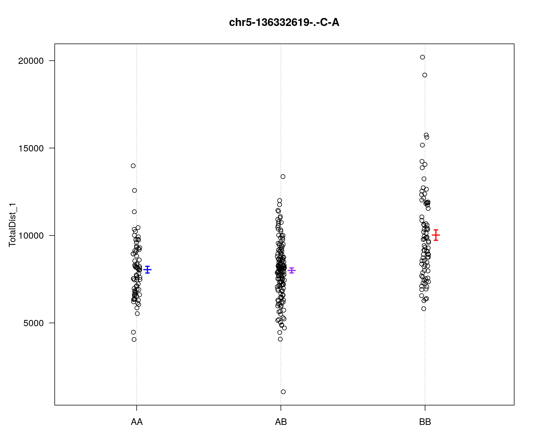
        fitqtl summary

Method: multiple imputation
Model:  normal phenotype
Number of observations : 309

Full model result
----------------------------------
Model formula: y ~ Q1 + Q2

       df         SS       MS      LOD     %var Pvalue(Chi2)   Pvalue(F)
Model   4  304259235 76064809 14.98603 20.01601 3.663736e-14 5.67324e-14
Error 304 1215819808  3999407
Total 308 1520079043


Drop one QTL at a time ANOVA table:
----------------------------------
        df Type III SS   LOD   %var F value Pvalue(Chi2) Pvalue(F)
5@76.0   2   211871869 10.78 13.938  26.488        0.000  2.49e-11 ***
14@36.1  2    58248627  3.14  3.832   7.282        0.001  0.000814 ***
---
Signif. codes:  0 '***' 0.001 '**' 0.01 '*' 0.05 '.' 0.1 ' ' 1


        fitqtl summary

Method: multiple imputation
Model:  normal phenotype
Number of observations : 309

Full model result
----------------------------------
Model formula: y ~ Q1 + Q2

       df         SS       MS      LOD     %var Pvalue(Chi2)   Pvalue(F)
Model   4  304259235 76064809 14.98603 20.01601 3.663736e-14 5.67324e-14
Error 304 1215819808  3999407
Total 308 1520079043


Estimated effects:
-----------------
              est      SE      t
Intercept 8572.65  116.00 73.901
5@76.0a    962.59  159.30  6.042
5@76.0d   -892.10  231.13 -3.860
14@36.1a   648.44  174.86  3.708
14@36.1d    67.35  232.36  0.290

[1] "To assess the possibility of an interaction between the two QTL"

        fitqtl summary

Method: multiple imputation
Model:  normal phenotype
Number of observations : 309

Full model result
----------------------------------
Model formula: y ~ Q1 + Q2 + Q1:Q2

       df         SS       MS      LOD     %var Pvalue(Chi2)    Pvalue(F)
Model   8  310801808 38850226 15.34808 20.44642 3.597012e-12 6.794232e-12
Error 300 1209277236  4030924
Total 308 1520079043


Drop one QTL at a time ANOVA table:
----------------------------------
               df Type III SS    LOD    %var F value Pvalue(Chi2) Pvalue(F)
5@76.0          6   218414441 11.141 14.3686  9.0308        0.000  4.41e-09 ***
14@36.1         6    64791200  3.502  4.2624  2.6789        0.013    0.0151 *
5@76.0:14@36.1  4     6542573  0.362  0.4304  0.4058        0.797    0.8045
---
Signif. codes:  0 '***' 0.001 '**' 0.01 '*' 0.05 '.' 0.1 ' ' 1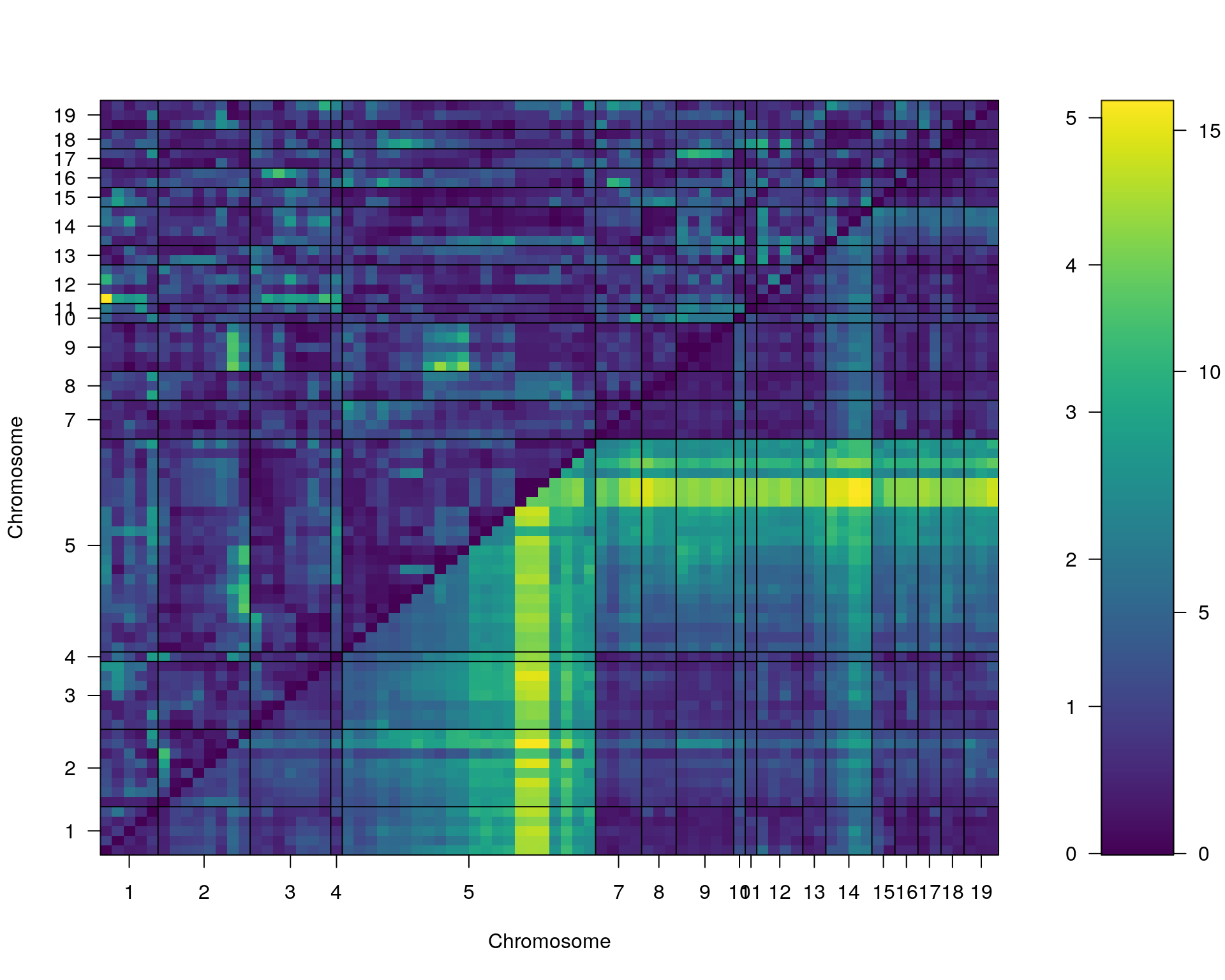
[1] "TotalDist_2"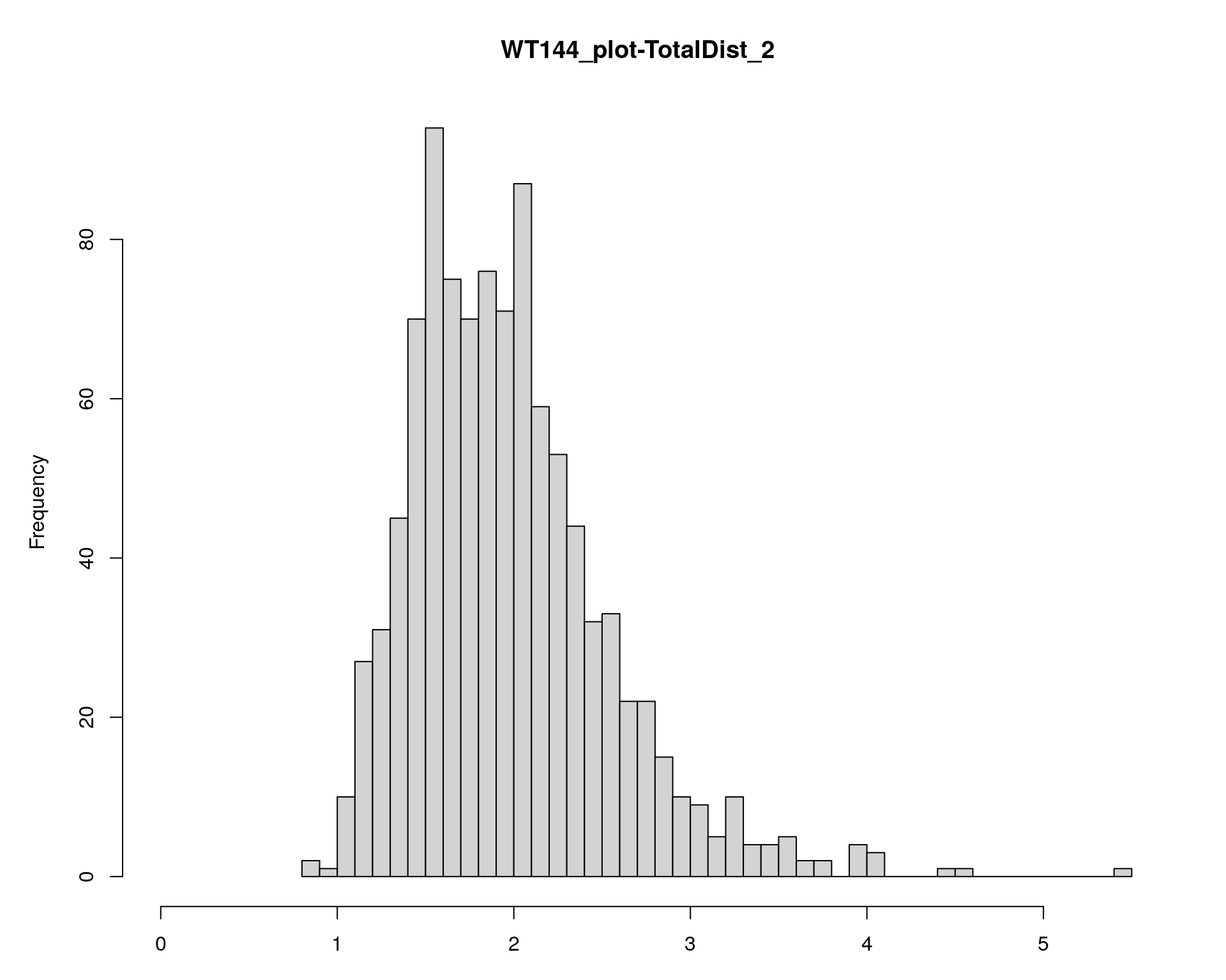
                     chr  pos   lod
chr2-137498061-.-T-A   2 67.9  3.60
chr5-136332619-.-C-A   5 76.0 24.45
chr14-69691477-.-G-T  14 36.1  4.61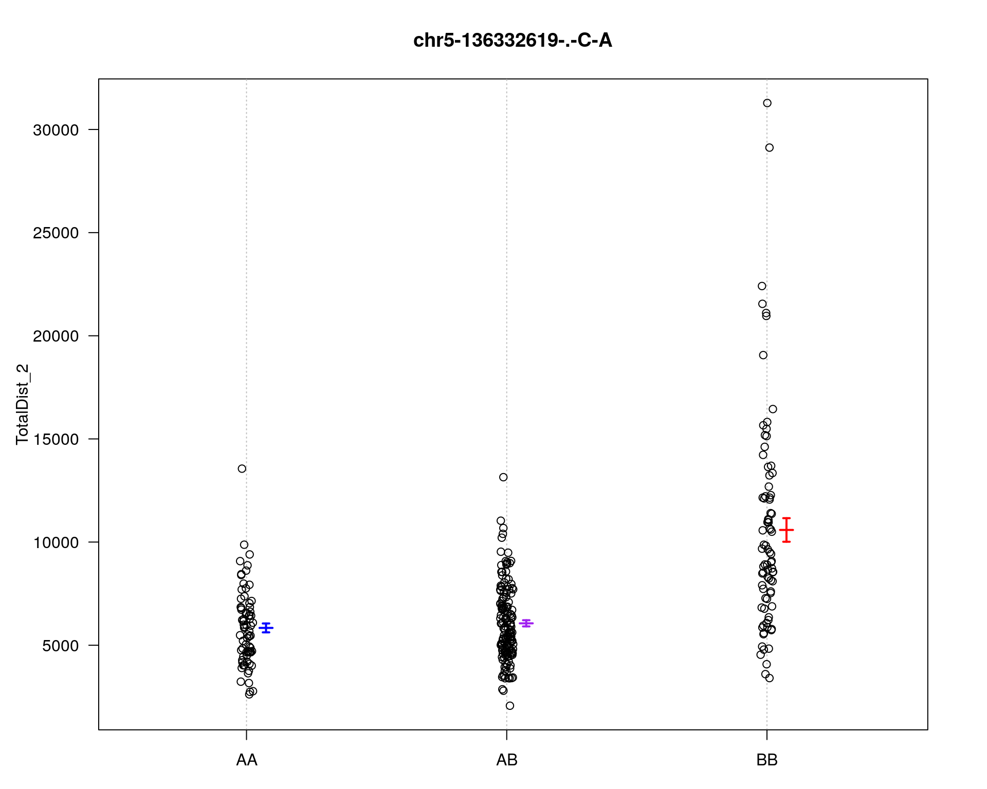
        fitqtl summary

Method: multiple imputation
Model:  normal phenotype
Number of observations : 308

Full model result
----------------------------------
Model formula: y ~ Q1 + Q2

       df         SS        MS      LOD     %var Pvalue(Chi2) Pvalue(F)
Model   4 1416731750 354182938 26.93405 33.14967            0         0
Error 303 2857011269   9429080
Total 307 4273743020


Drop one QTL at a time ANOVA table:
----------------------------------
        df Type III SS    LOD   %var F value Pvalue(Chi2) Pvalue(F)
5@76.0   2   1.134e+09 22.362 26.542  60.151        0.000   < 2e-16 ***
14@36.1  2   1.434e+08  3.275  3.355   7.604        0.001  0.000599 ***
---
Signif. codes:  0 '***' 0.001 '**' 0.01 '*' 0.05 '.' 0.1 ' ' 1


        fitqtl summary

Method: multiple imputation
Model:  normal phenotype
Number of observations : 308

Full model result
----------------------------------
Model formula: y ~ Q1 + Q2

       df         SS        MS      LOD     %var Pvalue(Chi2) Pvalue(F)
Model   4 1416731750 354182938 26.93405 33.14967            0         0
Error 303 2857011269   9429080
Total 307 4273743020


Estimated effects:
-----------------
              est      SE      t
Intercept  7248.6   178.6 40.590
5@76.0a    2302.4   245.2  9.390
5@76.0d   -1911.2   355.1 -5.382
14@36.1a   1047.8   269.6  3.886
14@36.1d   -347.5   357.7 -0.971

[1] "To assess the possibility of an interaction between the two QTL"

        fitqtl summary

Method: multiple imputation
Model:  normal phenotype
Number of observations : 308

Full model result
----------------------------------
Model formula: y ~ Q1 + Q2 + Q1:Q2

       df         SS        MS      LOD    %var Pvalue(Chi2) Pvalue(F)
Model   8 1497634877 187204360 28.85529 35.0427            0         0
Error 299 2776108143   9284643
Total 307 4273743020


Drop one QTL at a time ANOVA table:
----------------------------------
               df Type III SS    LOD   %var F value Pvalue(Chi2) Pvalue(F)
5@76.0          6   1.215e+09 24.283 28.435  21.814        0.000   < 2e-16 ***
14@36.1         6   2.243e+08  5.197  5.248   4.026        0.001  0.000677 ***
5@76.0:14@36.1  4   8.090e+07  1.921  1.893   2.178        0.065  0.071399 .
---
Signif. codes:  0 '***' 0.001 '**' 0.01 '*' 0.05 '.' 0.1 ' ' 1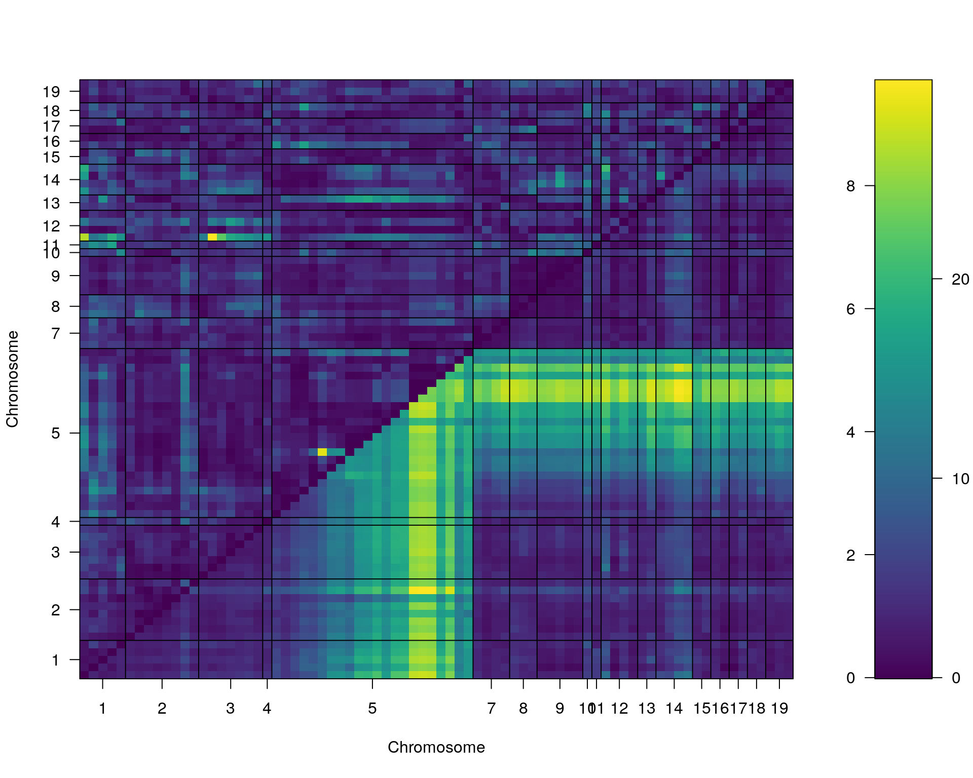
[1] "TotalDist_3"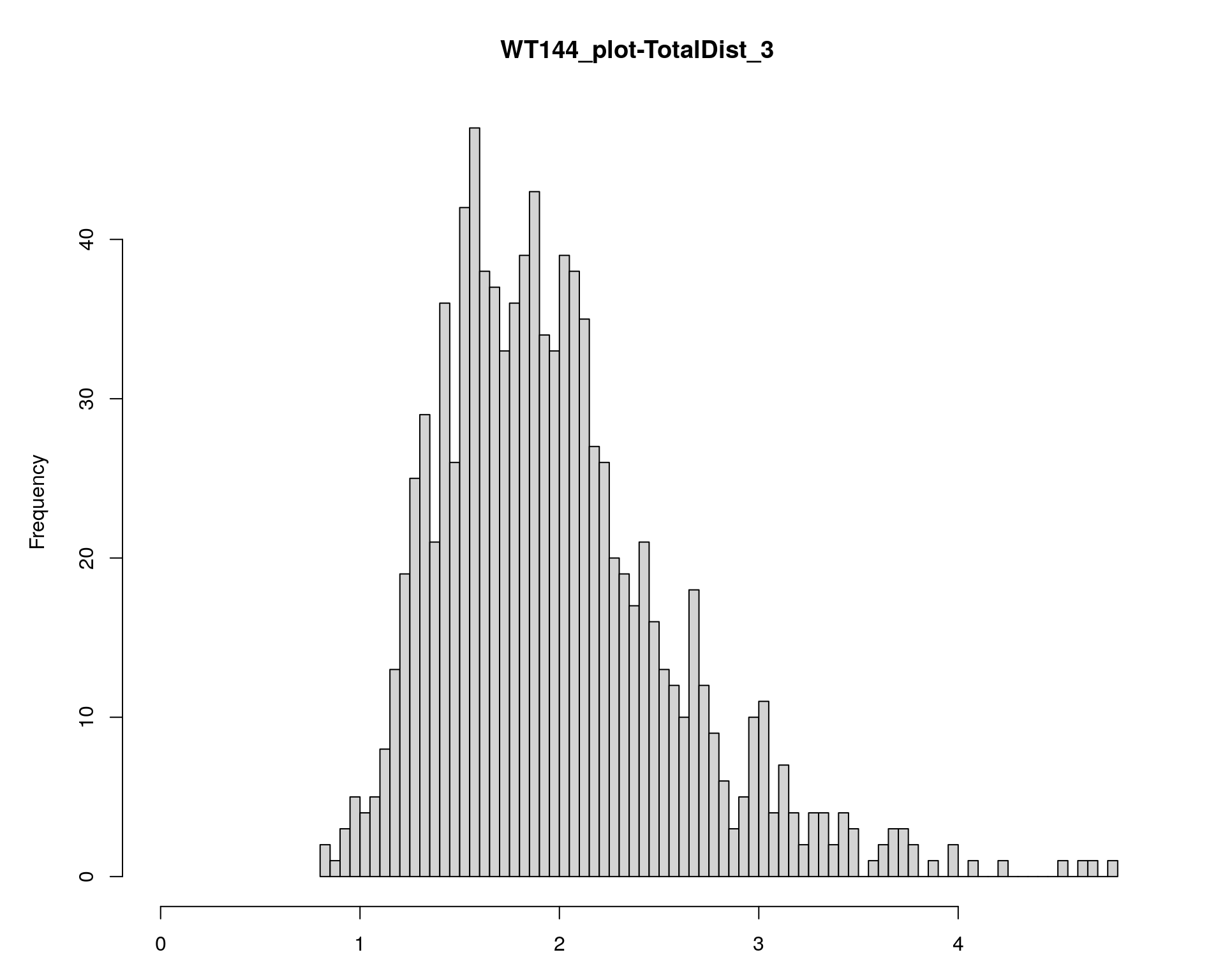
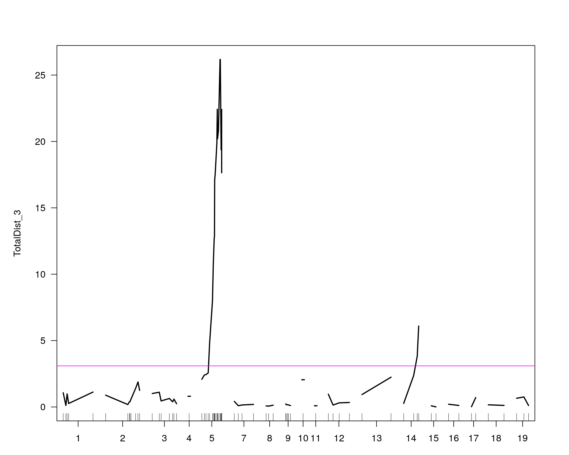
                     chr  pos   lod
chr5-136332619-.-C-A   5 76.0 26.18
chr14-69691477-.-G-T  14 36.1  6.09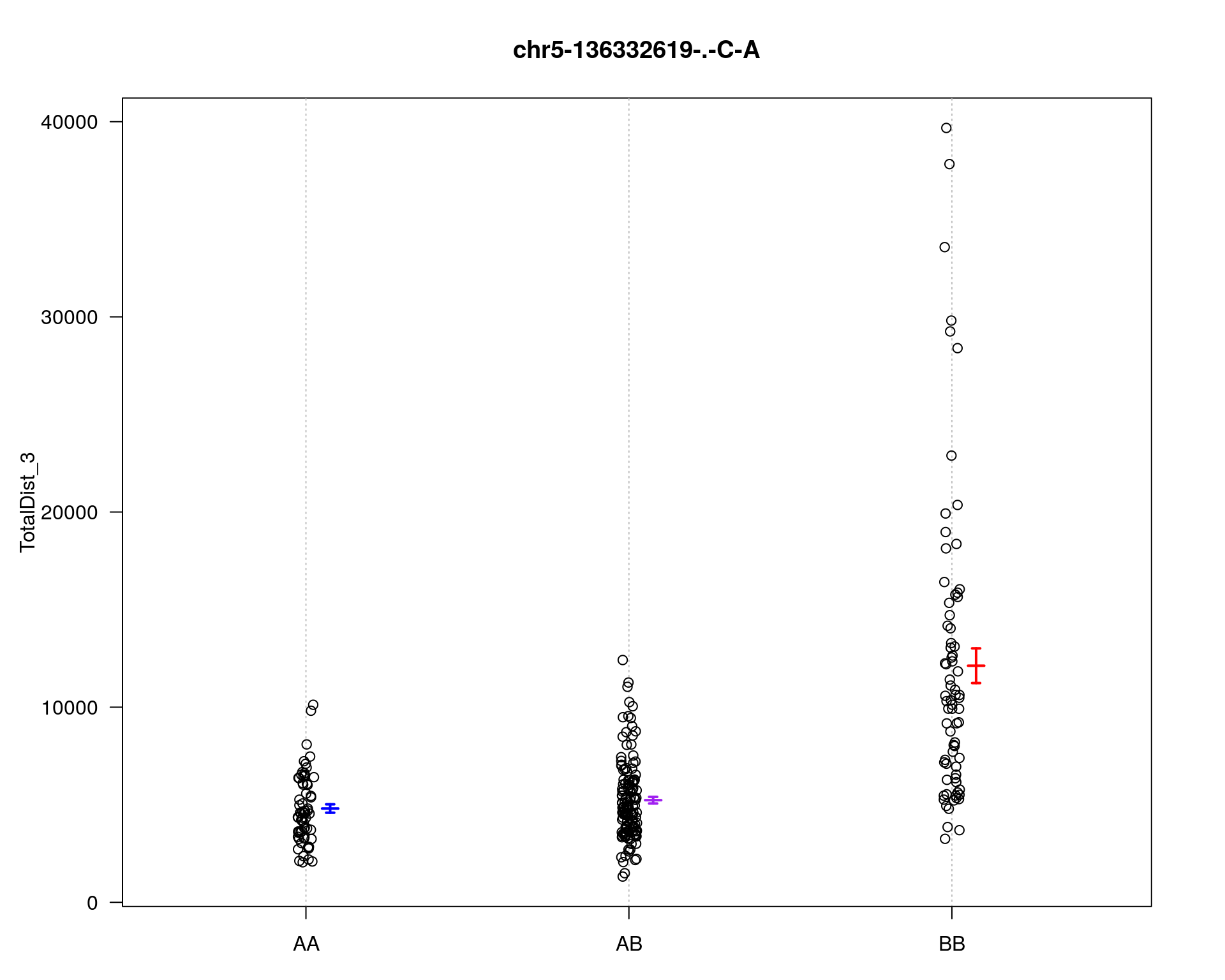
        fitqtl summary

Method: multiple imputation
Model:  normal phenotype
Number of observations : 281

Full model result
----------------------------------
Model formula: y ~ Q1 + Q2

       df         SS        MS      LOD     %var Pvalue(Chi2) Pvalue(F)
Model   4 3170972617 792743154 31.45631 40.28112            0         0
Error 276 4701133507  17033092
Total 280 7872106124


Drop one QTL at a time ANOVA table:
----------------------------------
        df Type III SS    LOD   %var F value Pvalue(Chi2) Pvalue(F)
5@76.0   2   2.423e+09 25.367 30.783   71.13            0   < 2e-16 ***
14@36.1  2   4.478e+08  5.552  5.689   13.15            0  3.52e-06 ***
---
Signif. codes:  0 '***' 0.001 '**' 0.01 '*' 0.05 '.' 0.1 ' ' 1


        fitqtl summary

Method: multiple imputation
Model:  normal phenotype
Number of observations : 281

Full model result
----------------------------------
Model formula: y ~ Q1 + Q2

       df         SS        MS      LOD     %var Pvalue(Chi2) Pvalue(F)
Model   4 3170972617 792743154 31.45631 40.28112            0         0
Error 276 4701133507  17033092
Total 280 7872106124


Estimated effects:
-----------------
              est      SE      t
Intercept  7106.2   251.6 28.249
5@76.0a    3548.9   349.2 10.162
5@76.0d   -2908.4   497.5 -5.846
14@36.1a   1818.8   380.1  4.785
14@36.1d  -1335.6   503.4 -2.653

[1] "To assess the possibility of an interaction between the two QTL"

        fitqtl summary

Method: multiple imputation
Model:  normal phenotype
Number of observations : 281

Full model result
----------------------------------
Model formula: y ~ Q1 + Q2 + Q1:Q2

       df         SS        MS      LOD     %var Pvalue(Chi2) Pvalue(F)
Model   8 3558447363 444805920 36.70494 45.20324            0         0
Error 272 4313658761  15859040
Total 280 7872106124


Drop one QTL at a time ANOVA table:
----------------------------------
               df Type III SS    LOD   %var F value Pvalue(Chi2) Pvalue(F)
5@76.0          6   2.811e+09 30.615 35.705  29.539            0   < 2e-16 ***
14@36.1         6   8.353e+08 10.801 10.611   8.778            0  9.41e-09 ***
5@76.0:14@36.1  4   3.875e+08  5.249  4.922   6.108            0  0.000101 ***
---
Signif. codes:  0 '***' 0.001 '**' 0.01 '*' 0.05 '.' 0.1 ' ' 1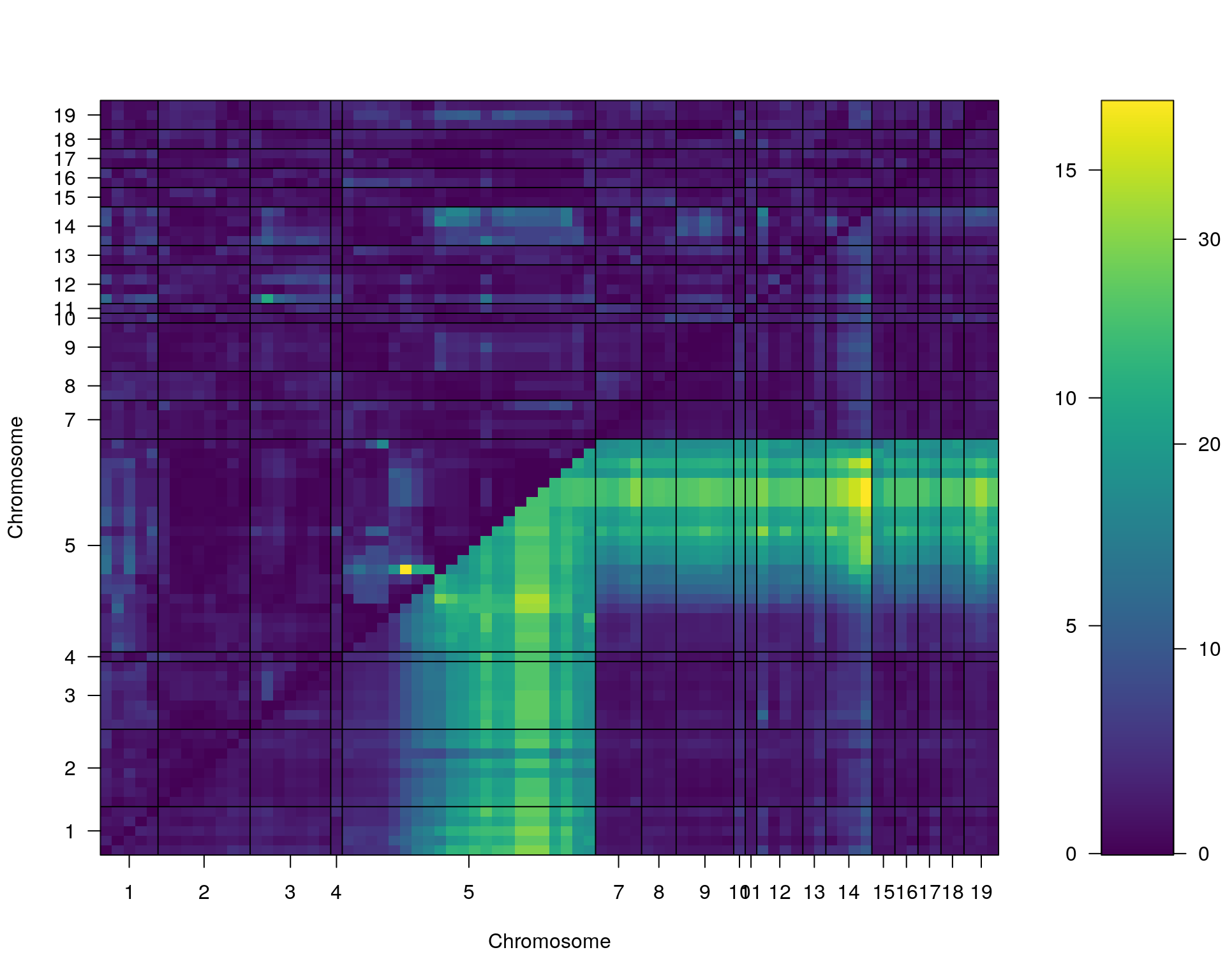
[1] "base.y"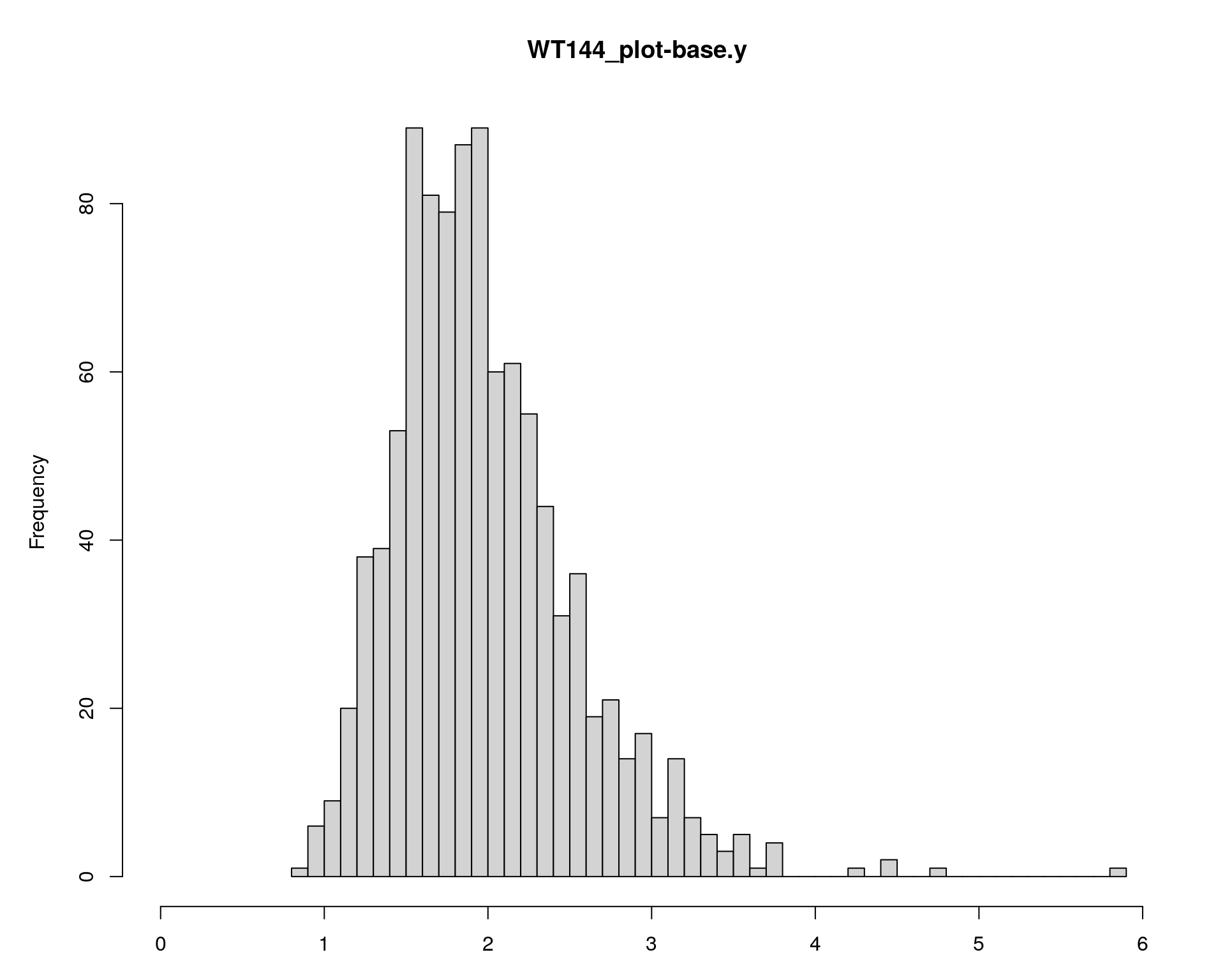
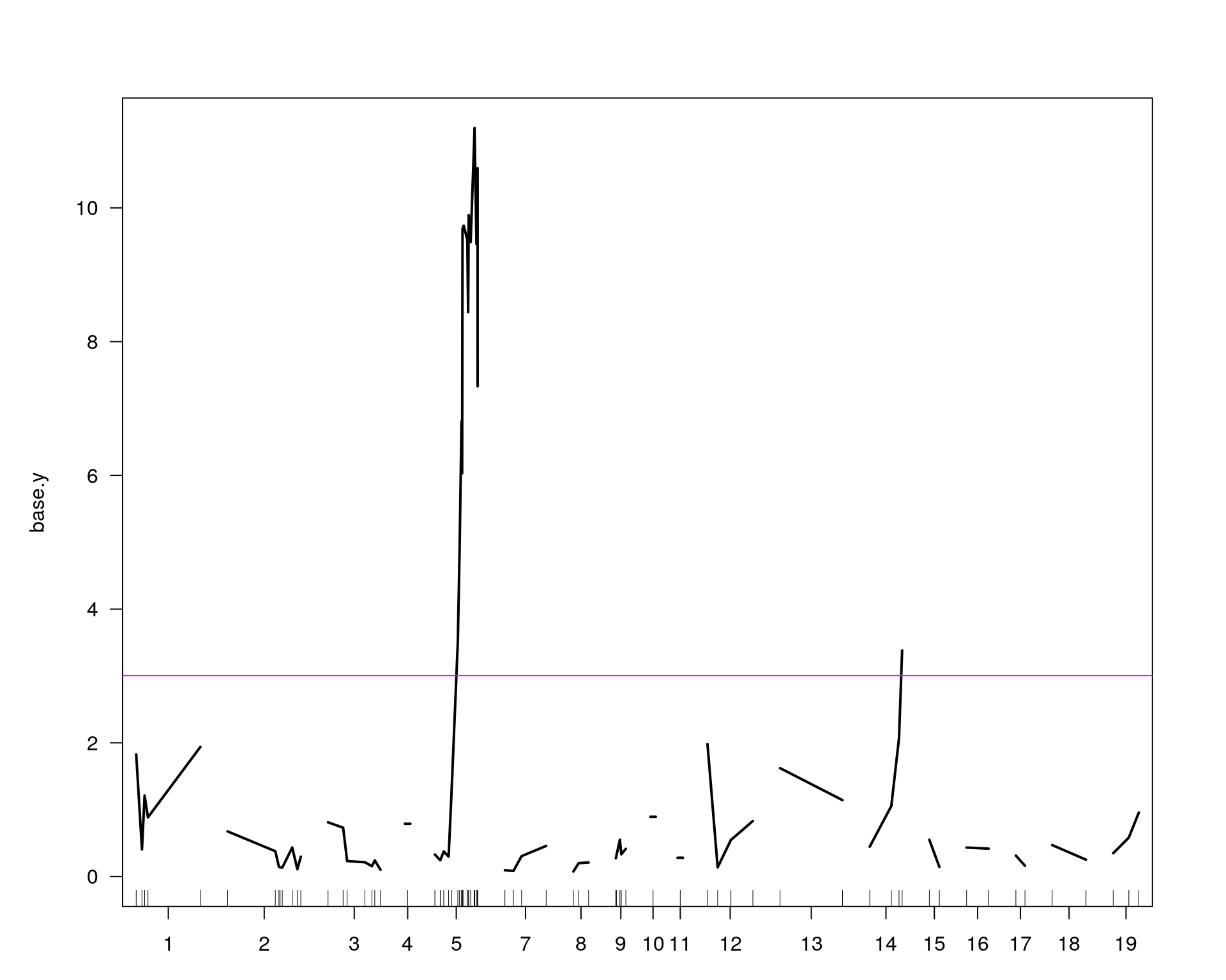
                     chr  pos   lod
chr5-136332619-.-C-A   5 76.0 11.20
chr14-69691477-.-G-T  14 36.1  3.38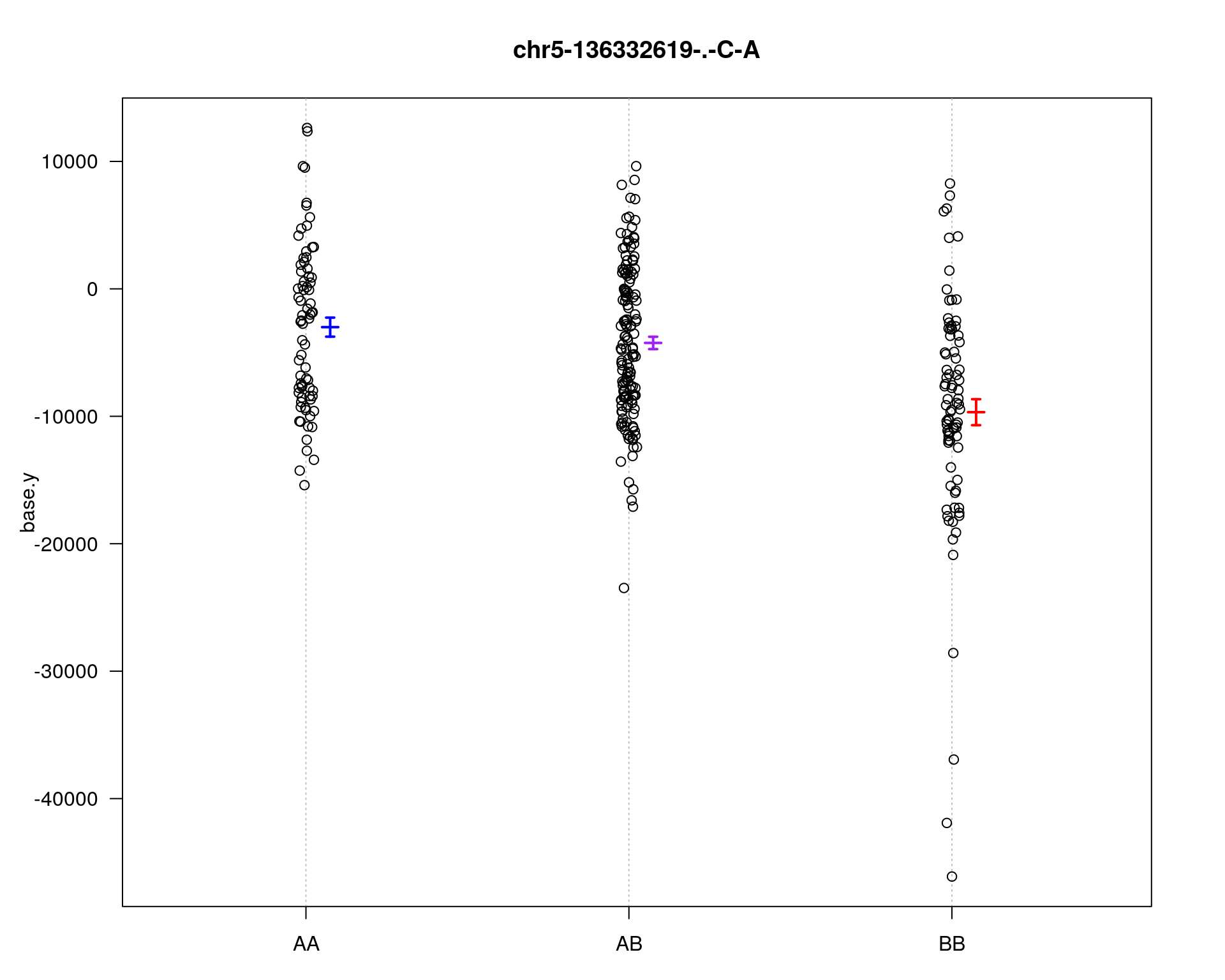
        fitqtl summary

Method: multiple imputation
Model:  normal phenotype
Number of observations : 307

Full model result
----------------------------------
Model formula: y ~ Q1 + Q2

       df          SS        MS      LOD     %var Pvalue(Chi2)    Pvalue(F)
Model   4  2303684755 575921189 9.402448 13.15471 8.966422e-09 1.175103e-08
Error 302 15208557648  50359462
Total 306 17512242403


Drop one QTL at a time ANOVA table:
----------------------------------
        df Type III SS    LOD   %var F value Pvalue(Chi2) Pvalue(F)
5@76.0   2   1.848e+09 7.6458 10.554  18.350        0.000  3.01e-08 ***
14@36.1  2   2.208e+08 0.9609  1.261   2.192        0.109     0.113
---
Signif. codes:  0 '***' 0.001 '**' 0.01 '*' 0.05 '.' 0.1 ' ' 1


        fitqtl summary

Method: multiple imputation
Model:  normal phenotype
Number of observations : 307

Full model result
----------------------------------
Model formula: y ~ Q1 + Q2

       df          SS        MS      LOD     %var Pvalue(Chi2)    Pvalue(F)
Model   4  2303684755 575921189 9.402448 13.15471 8.966422e-09 1.175103e-08
Error 302 15208557648  50359462
Total 306 17512242403


Estimated effects:
-----------------
              est      SE       t
Intercept -5438.3   412.5 -13.184
5@76.0a   -3187.9   569.7  -5.596
5@76.0d    1760.7   823.9   2.137
14@36.1a  -1158.4   622.3  -1.862
14@36.1d   1024.2   827.5   1.238

[1] "To assess the possibility of an interaction between the two QTL"

        fitqtl summary

Method: multiple imputation
Model:  normal phenotype
Number of observations : 307

Full model result
----------------------------------
Model formula: y ~ Q1 + Q2 + Q1:Q2

       df          SS        MS      LOD     %var Pvalue(Chi2)    Pvalue(F)
Model   8  2837695855 354711982 11.78528 16.20407 6.110339e-09 9.850676e-09
Error 298 14674546548  49243445
Total 306 17512242403


Drop one QTL at a time ANOVA table:
----------------------------------
               df Type III SS    LOD   %var F value Pvalue(Chi2) Pvalue(F)
5@76.0          6   2.382e+09 10.029 13.603   8.063        0.000  4.42e-08 ***
14@36.1         6   7.548e+08  3.344  4.310   2.555        0.017    0.0199 *
5@76.0:14@36.1  4   5.340e+08  2.383  3.049   2.711        0.027    0.0303 *
---
Signif. codes:  0 '***' 0.001 '**' 0.01 '*' 0.05 '.' 0.1 ' ' 1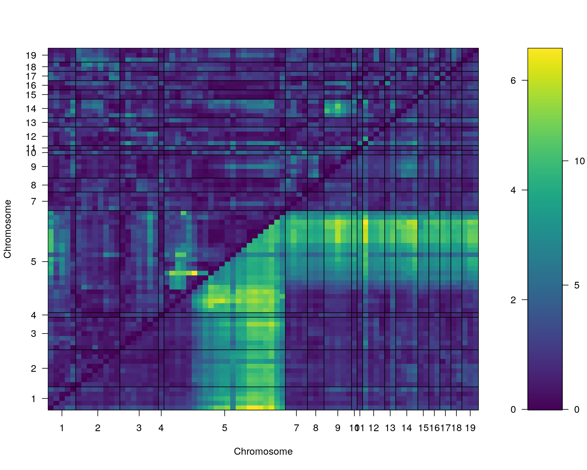
[1] "TestAge.y"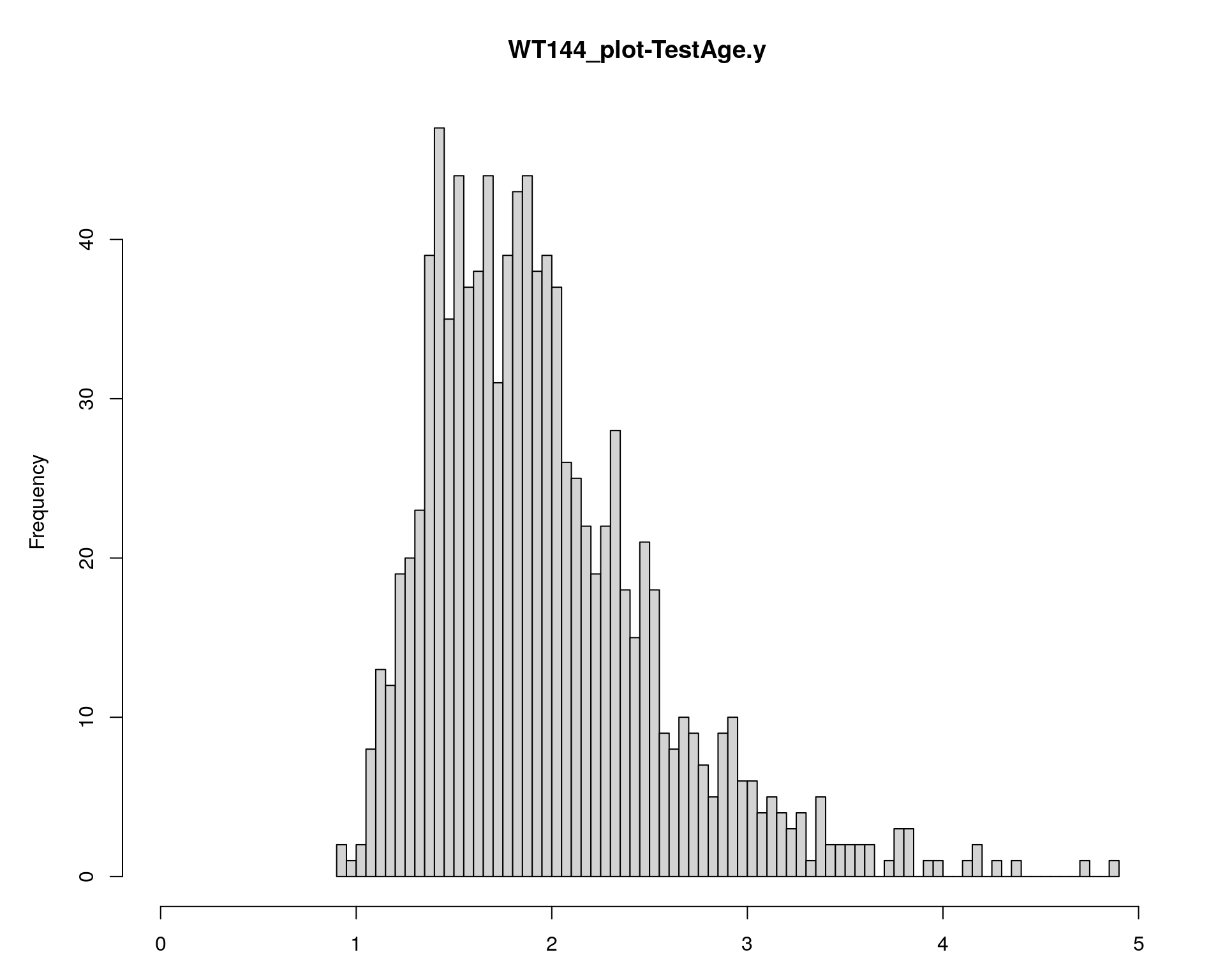

                     chr  pos   lod
chr5-136332619-.-C-A   5 76.0 21.31
chr14-69691477-.-G-T  14 36.1  5.34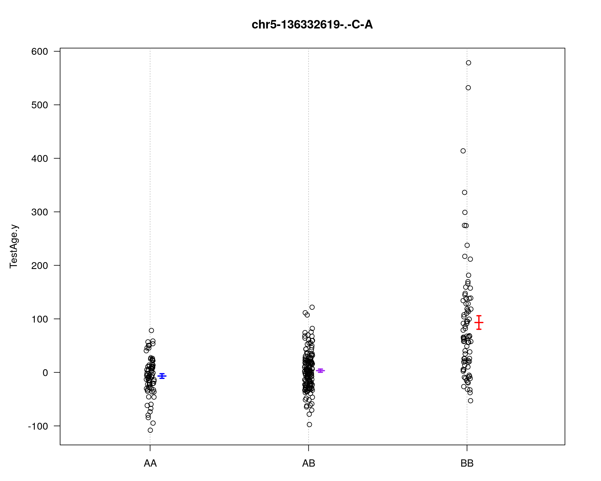
        fitqtl summary

Method: multiple imputation
Model:  normal phenotype
Number of observations : 307

Full model result
----------------------------------
Model formula: y ~ Q1 + Q2

       df        SS         MS      LOD     %var Pvalue(Chi2) Pvalue(F)
Model   4  608155.7 152038.921 25.48727 31.77255            0         0
Error 302 1305936.1   4324.292
Total 306 1914091.7


Drop one QTL at a time ANOVA table:
----------------------------------
        df Type III SS    LOD  %var F value Pvalue(Chi2) Pvalue(F)
5@76.0   2      460494 20.135 24.06  53.245            0   < 2e-16 ***
14@36.1  2       80200  3.973  4.19   9.273            0  0.000123 ***
---
Signif. codes:  0 '***' 0.001 '**' 0.01 '*' 0.05 '.' 0.1 ' ' 1


        fitqtl summary

Method: multiple imputation
Model:  normal phenotype
Number of observations : 307

Full model result
----------------------------------
Model formula: y ~ Q1 + Q2

       df        SS         MS      LOD     %var Pvalue(Chi2) Pvalue(F)
Model   4  608155.7 152038.921 25.48727 31.77255            0         0
Error 302 1305936.1   4324.292
Total 306 1914091.7


Estimated effects:
-----------------
              est      SE      t
Intercept  26.175   3.830  6.834
5@76.0a    47.811   5.272  9.069
5@76.0d   -35.014   7.624 -4.593
14@36.1a   21.094   5.791  3.642
14@36.1d  -21.931   7.675 -2.858

[1] "To assess the possibility of an interaction between the two QTL"

        fitqtl summary

Method: multiple imputation
Model:  normal phenotype
Number of observations : 307

Full model result
----------------------------------
Model formula: y ~ Q1 + Q2 + Q1:Q2

       df      SS        MS      LOD     %var Pvalue(Chi2) Pvalue(F)
Model   8  718668 89833.502 31.38167 37.54616            0         0
Error 298 1195424  4011.489
Total 306 1914092


Drop one QTL at a time ANOVA table:
----------------------------------
               df Type III SS    LOD   %var F value Pvalue(Chi2) Pvalue(F)
5@76.0          6      571007 26.030 29.832  23.724            0   < 2e-16 ***
14@36.1         6      190712  9.868  9.964   7.924            0  6.15e-08 ***
5@76.0:14@36.1  4      110512  5.894  5.774   6.887            0  2.58e-05 ***
---
Signif. codes:  0 '***' 0.001 '**' 0.01 '*' 0.05 '.' 0.1 ' ' 1
[1] "Intercept"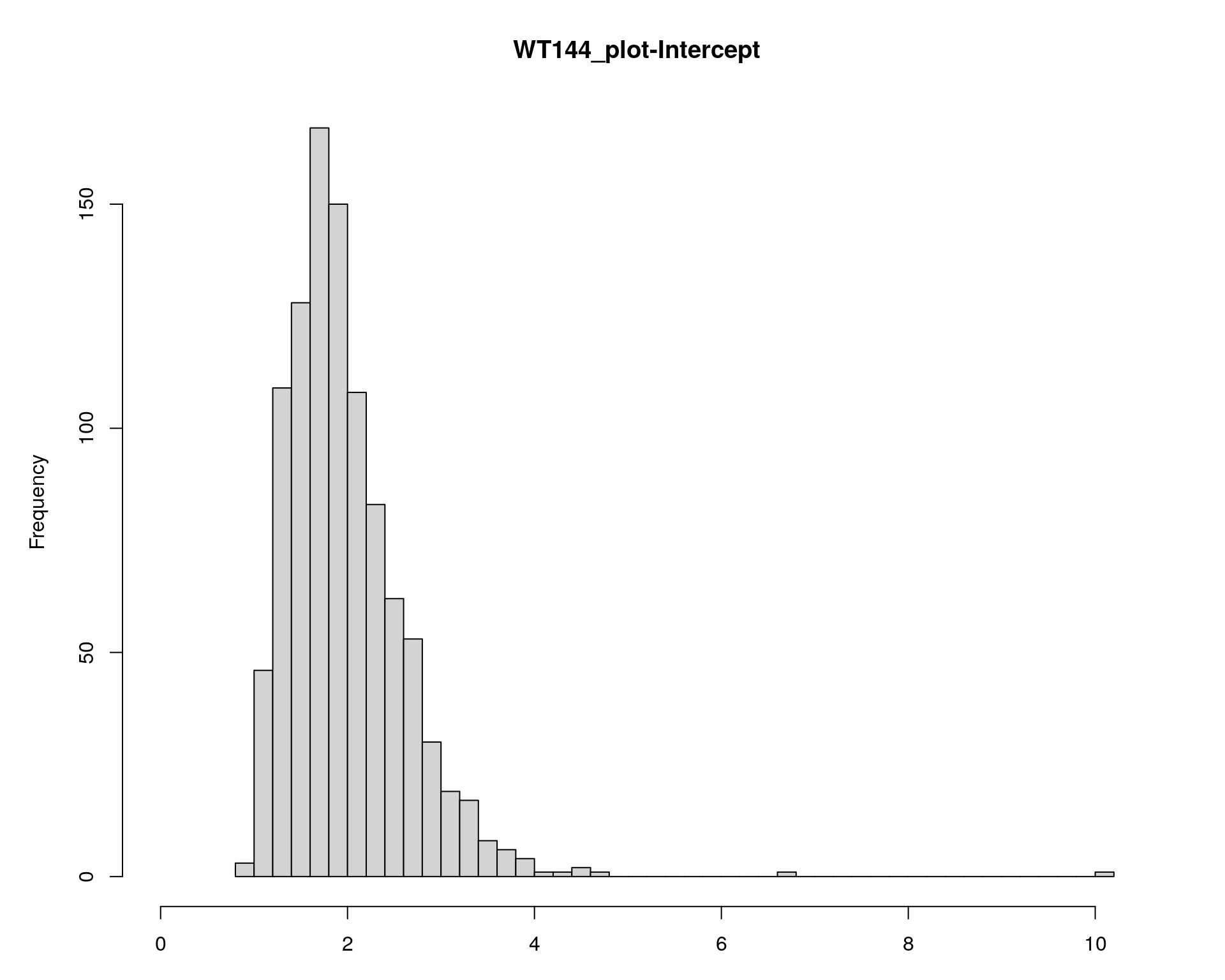
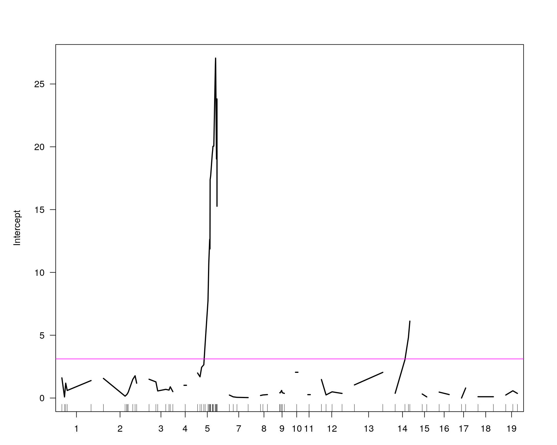
                     chr  pos   lod
chr5-136332619-.-C-A   5 76.0 27.06
chr14-69691477-.-G-T  14 36.1  6.12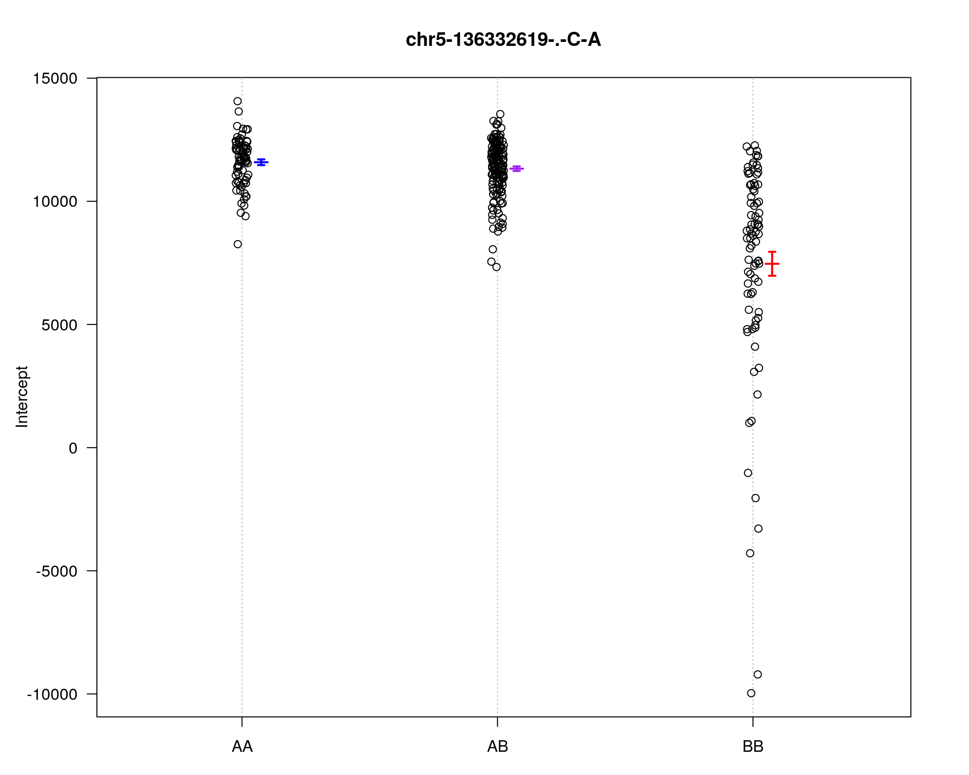
        fitqtl summary

Method: multiple imputation
Model:  normal phenotype
Number of observations : 309

Full model result
----------------------------------
Model formula: y ~ Q1 + Q2

       df         SS        MS     LOD     %var Pvalue(Chi2) Pvalue(F)
Model   4 1076068514 269017128 31.4753 37.44293            0         0
Error 304 1797820892   5913885
Total 308 2873889406


Drop one QTL at a time ANOVA table:
----------------------------------
        df Type III SS    LOD   %var F value Pvalue(Chi2) Pvalue(F)
5@76.0   2   824376118 25.325 28.685   69.70            0   < 2e-16 ***
14@36.1  2   125661963  4.533  4.373   10.62            0  3.47e-05 ***
---
Signif. codes:  0 '***' 0.001 '**' 0.01 '*' 0.05 '.' 0.1 ' ' 1


        fitqtl summary

Method: multiple imputation
Model:  normal phenotype
Number of observations : 309

Full model result
----------------------------------
Model formula: y ~ Q1 + Q2

       df         SS        MS     LOD     %var Pvalue(Chi2) Pvalue(F)
Model   4 1076068514 269017128 31.4753 37.44293            0         0
Error 304 1797820892   5913885
Total 308 2873889406


Estimated effects:
-----------------
              est      SE       t
Intercept 10313.0   141.1  73.096
5@76.0a   -1975.3   193.9 -10.186
5@76.0d    1584.7   281.1   5.638
14@36.1a   -917.4   212.6  -4.315
14@36.1d    649.7   282.7   2.298

[1] "To assess the possibility of an interaction between the two QTL"

        fitqtl summary

Method: multiple imputation
Model:  normal phenotype
Number of observations : 309

Full model result
----------------------------------
Model formula: y ~ Q1 + Q2 + Q1:Q2

       df         SS        MS      LOD    %var Pvalue(Chi2) Pvalue(F)
Model   8 1201636454 150204557 36.33347 41.8122            0         0
Error 300 1672252953   5574177
Total 308 2873889406


Drop one QTL at a time ANOVA table:
----------------------------------
               df Type III SS    LOD   %var F value Pvalue(Chi2) Pvalue(F)
5@76.0          6   949944058 30.184 33.054  28.403            0   < 2e-16 ***
14@36.1         6   251229903  9.391  8.742   7.512            0  1.63e-07 ***
5@76.0:14@36.1  4   125567940  4.858  4.369   5.632            0   0.00022 ***
---
Signif. codes:  0 '***' 0.001 '**' 0.01 '*' 0.05 '.' 0.1 ' ' 1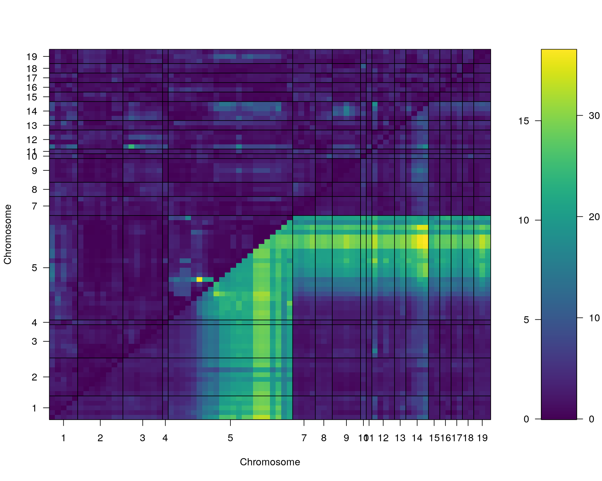
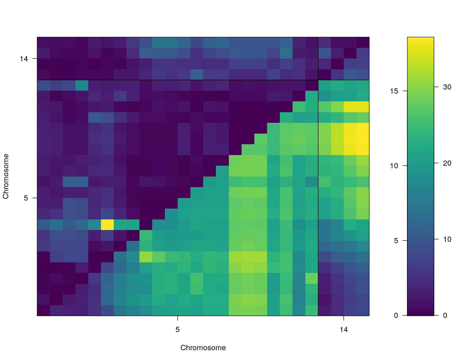
[1] "Slope"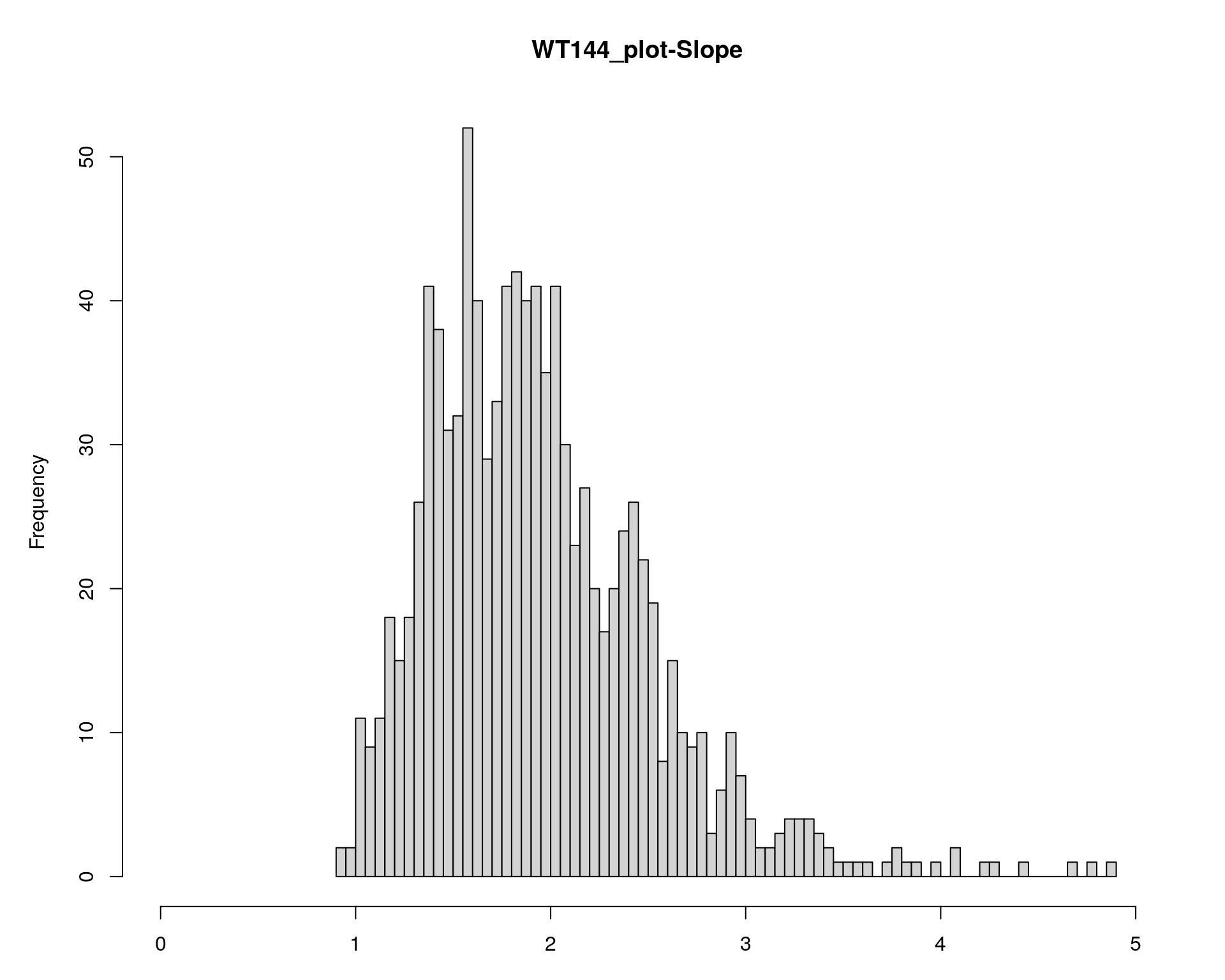
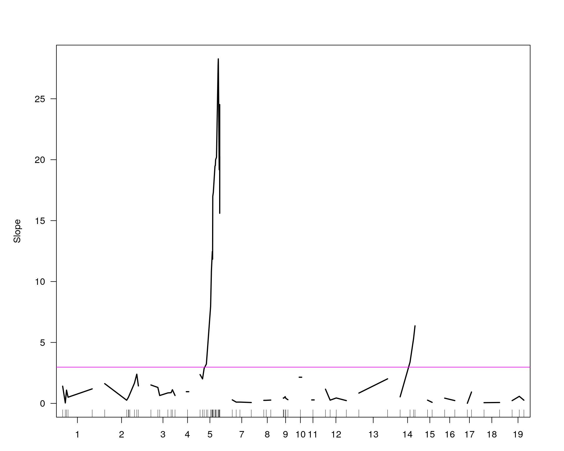
                     chr  pos   lod
chr5-136332619-.-C-A   5 76.0 28.27
chr14-69691477-.-G-T  14 36.1  6.37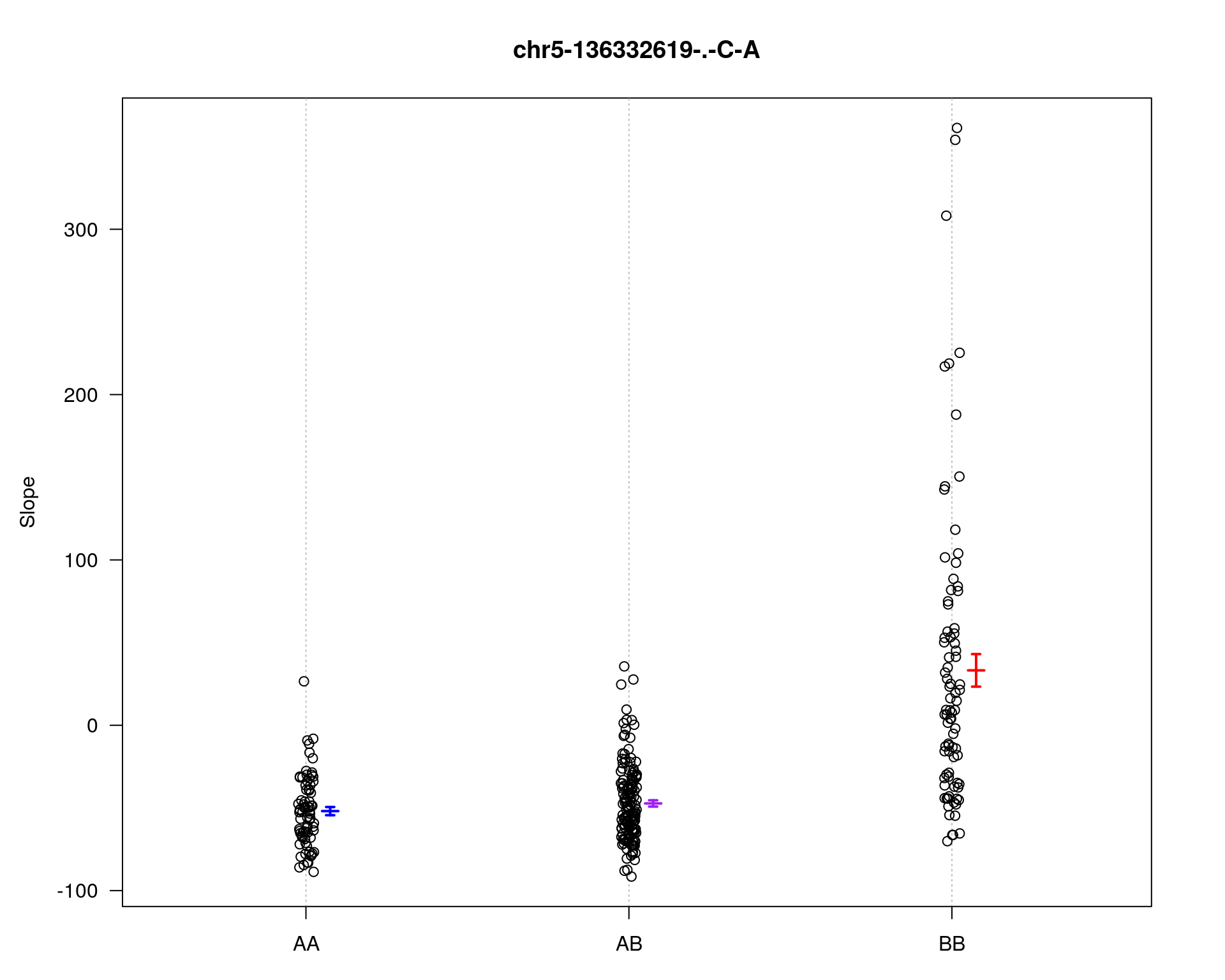
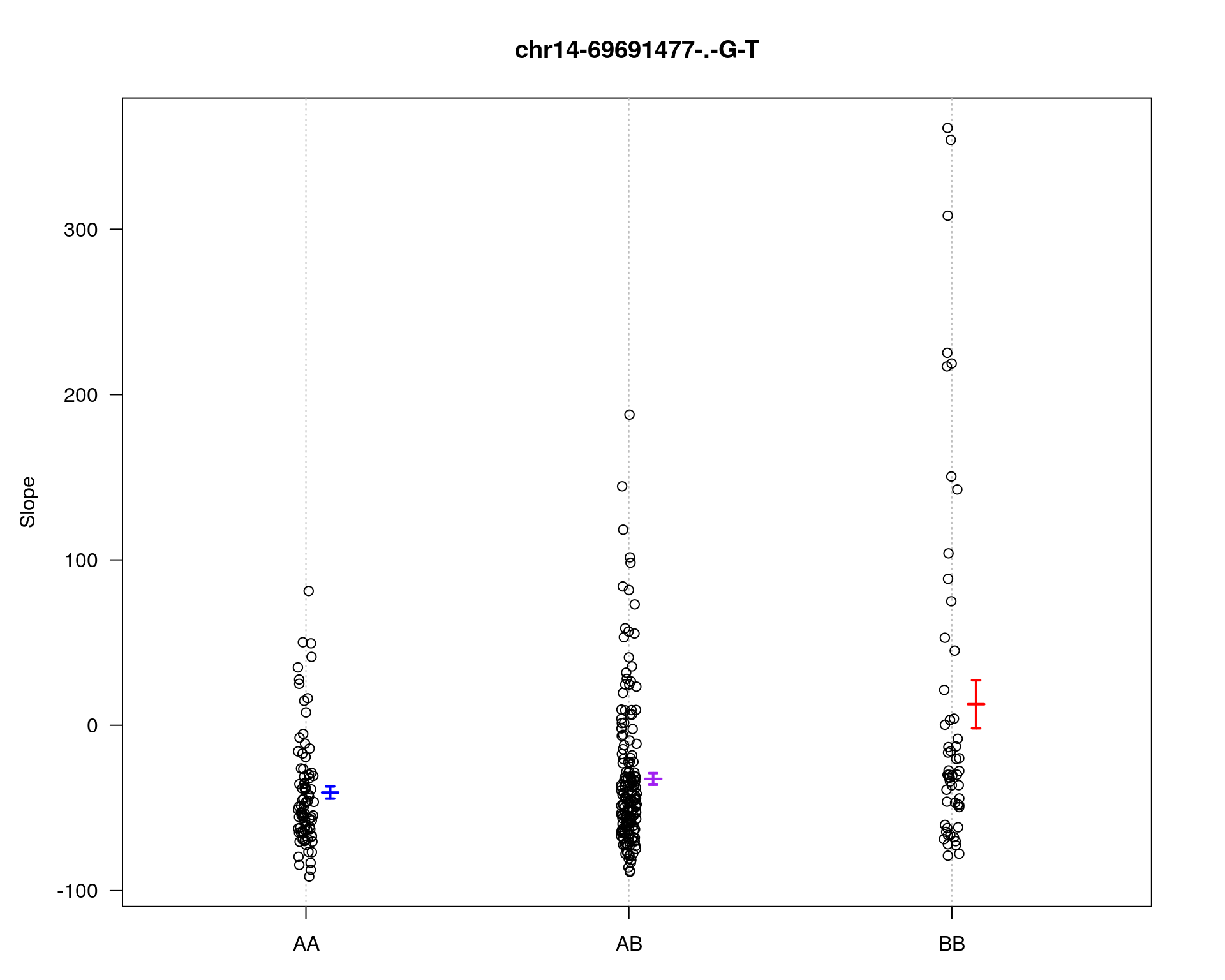
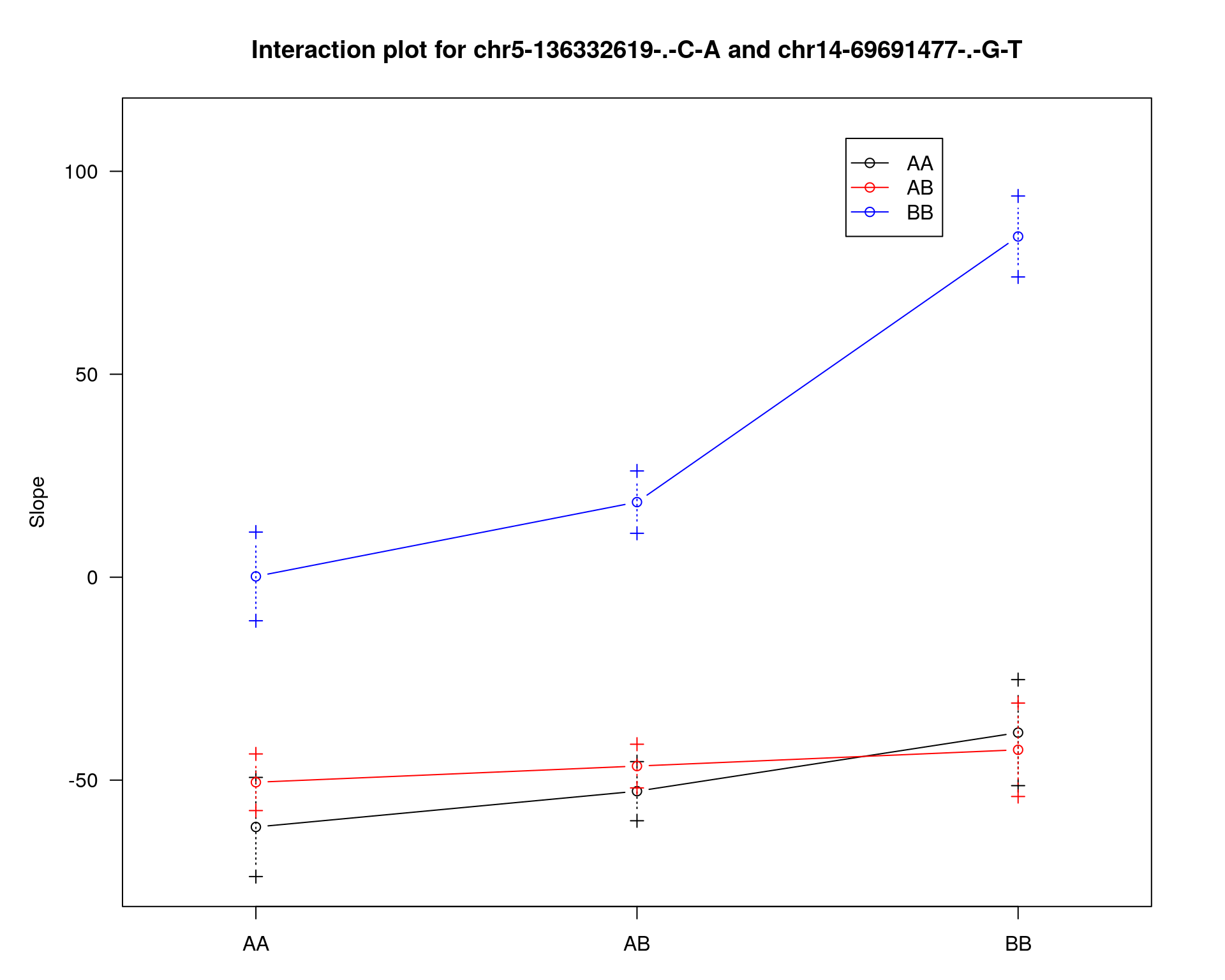
        fitqtl summary

Method: multiple imputation
Model:  normal phenotype
Number of observations : 309

Full model result
----------------------------------
Model formula: y ~ Q1 + Q2

       df        SS         MS      LOD     %var Pvalue(Chi2) Pvalue(F)
Model   4  464945.0 116236.249 32.79274 38.65922            0         0
Error 304  737730.5   2426.745
Total 308 1202675.5


Drop one QTL at a time ANOVA table:
----------------------------------
        df Type III SS    LOD   %var F value Pvalue(Chi2) Pvalue(F)
5@76.0   2      355763 26.407 29.581   73.30            0   < 2e-16 ***
14@36.1  2       55109  4.834  4.582   11.35            0  1.76e-05 ***
---
Signif. codes:  0 '***' 0.001 '**' 0.01 '*' 0.05 '.' 0.1 ' ' 1


        fitqtl summary

Method: multiple imputation
Model:  normal phenotype
Number of observations : 309

Full model result
----------------------------------
Model formula: y ~ Q1 + Q2

       df        SS         MS      LOD     %var Pvalue(Chi2) Pvalue(F)
Model   4  464945.0 116236.249 32.79274 38.65922            0         0
Error 304  737730.5   2426.745
Total 308 1202675.5


Estimated effects:
-----------------
              est      SE      t
Intercept -26.036   2.858 -9.109
5@76.0a    40.839   3.926 10.401
5@76.0d   -33.302   5.693 -5.849
14@36.1a   19.778   4.309  4.590
14@36.1d  -11.531   5.726 -2.014

[1] "To assess the possibility of an interaction between the two QTL"

        fitqtl summary

Method: multiple imputation
Model:  normal phenotype
Number of observations : 309

Full model result
----------------------------------
Model formula: y ~ Q1 + Q2 + Q1:Q2

       df        SS        MS      LOD     %var Pvalue(Chi2) Pvalue(F)
Model   8  507552.7 63444.092 36.78443 42.20197            0         0
Error 300  695122.7  2317.076
Total 308 1202675.5


Drop one QTL at a time ANOVA table:
----------------------------------
               df Type III SS    LOD   %var F value Pvalue(Chi2) Pvalue(F)
5@76.0          6      398371 30.399 33.124  28.655        0.000   < 2e-16 ***
14@36.1         6       97717  8.826  8.125   7.029        0.000  5.17e-07 ***
5@76.0:14@36.1  4       42608  3.992  3.543   4.597        0.001   0.00129 **
---
Signif. codes:  0 '***' 0.001 '**' 0.01 '*' 0.05 '.' 0.1 ' ' 1

#plot all phenotypes
plot(out.mr[[6]], col= "blue", ylim = c(0, 30), ylab = "LOD score")
plot(out.mr[[7]], col= "red",   add=TRUE)
plot(out.mr[[3]], col= "green", add=TRUE)
plot(out.mr[[4]], col= "black",  add=TRUE)
plot(out.mr[[5]], col=  "purple", add=TRUE)
abline(h=3.2, col="red", lty=2, lwd=3)
# Add a legend
legend("topright",
       legend=c("Base", "TestAge", "TotalDist_1", "TotalDist_2", "TotalDist_3"),
       col=c("blue", "red", "green", "black", "purple"), lty=1, cex=0.8)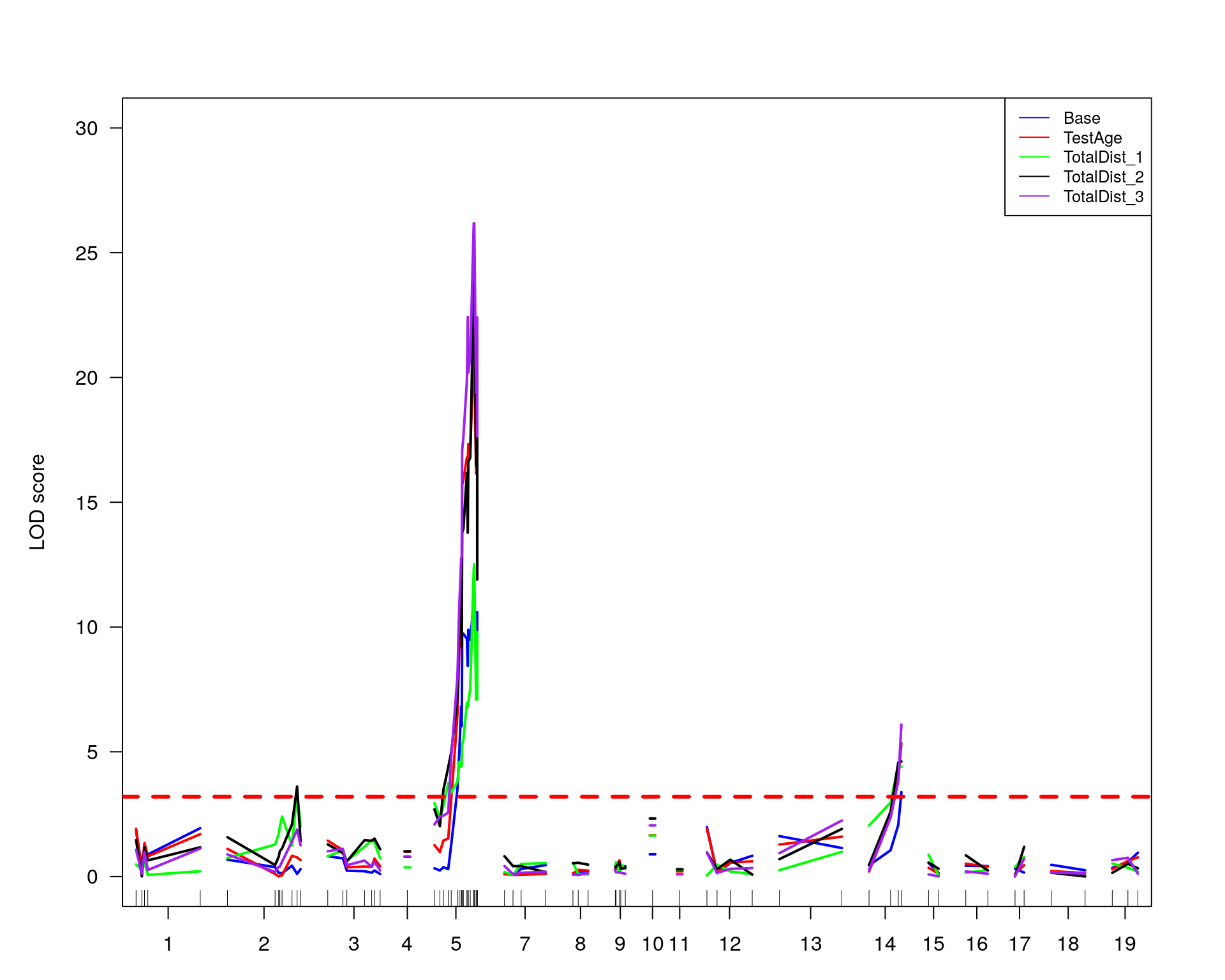
#only at chr 5 and 14
#plot all phenotypes
plot(out.mr[[6]], col= "blue", ylim = c(0, 30), ylab = "LOD score", chr = c(5, 14))
plot(out.mr[[7]], col= "red",   add=TRUE, chr = c(5, 14))
plot(out.mr[[3]], col= "green", add=TRUE, chr = c(5, 14))
plot(out.mr[[4]], col= "black",  add=TRUE, chr = c(5, 14))
plot(out.mr[[5]], col=  "purple", add=TRUE, chr = c(5, 14))
abline(h=3.2, col="red", lty=2, lwd=3)
# Add a legend
legend("topright",
       legend=c("Base", "TestAge", "TotalDist_1", "TotalDist_2", "TotalDist_3"),
       col=c("blue", "red", "green", "black", "purple"), lty=1, cex=0.8)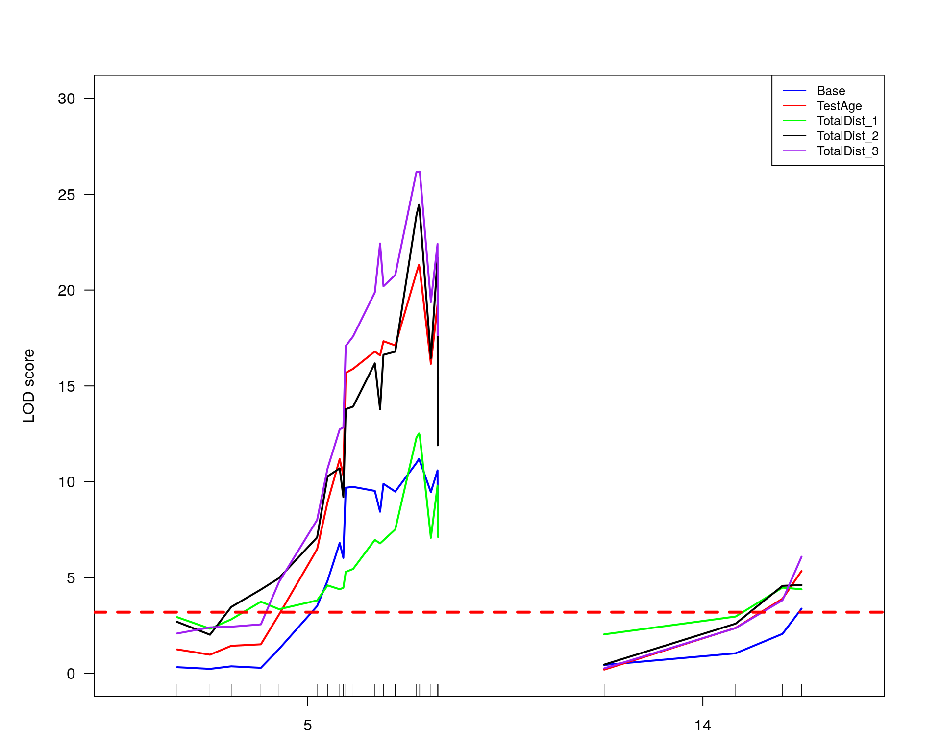
#plot phenotypes: slope and totaldistance3
plot(out.mr[[9]], col= "blue", ylim = c(0, 30), ylab = "LOD score")
plot(out.mr[[5]], col=  "green", add=TRUE)
abline(h=3.2, col="red", lty=2, lwd=3)
# Add a legend
legend("topright",
       legend=c("Slope", "TotalDist"),
       col=c("blue", "green"), lty=1, cex=0.8)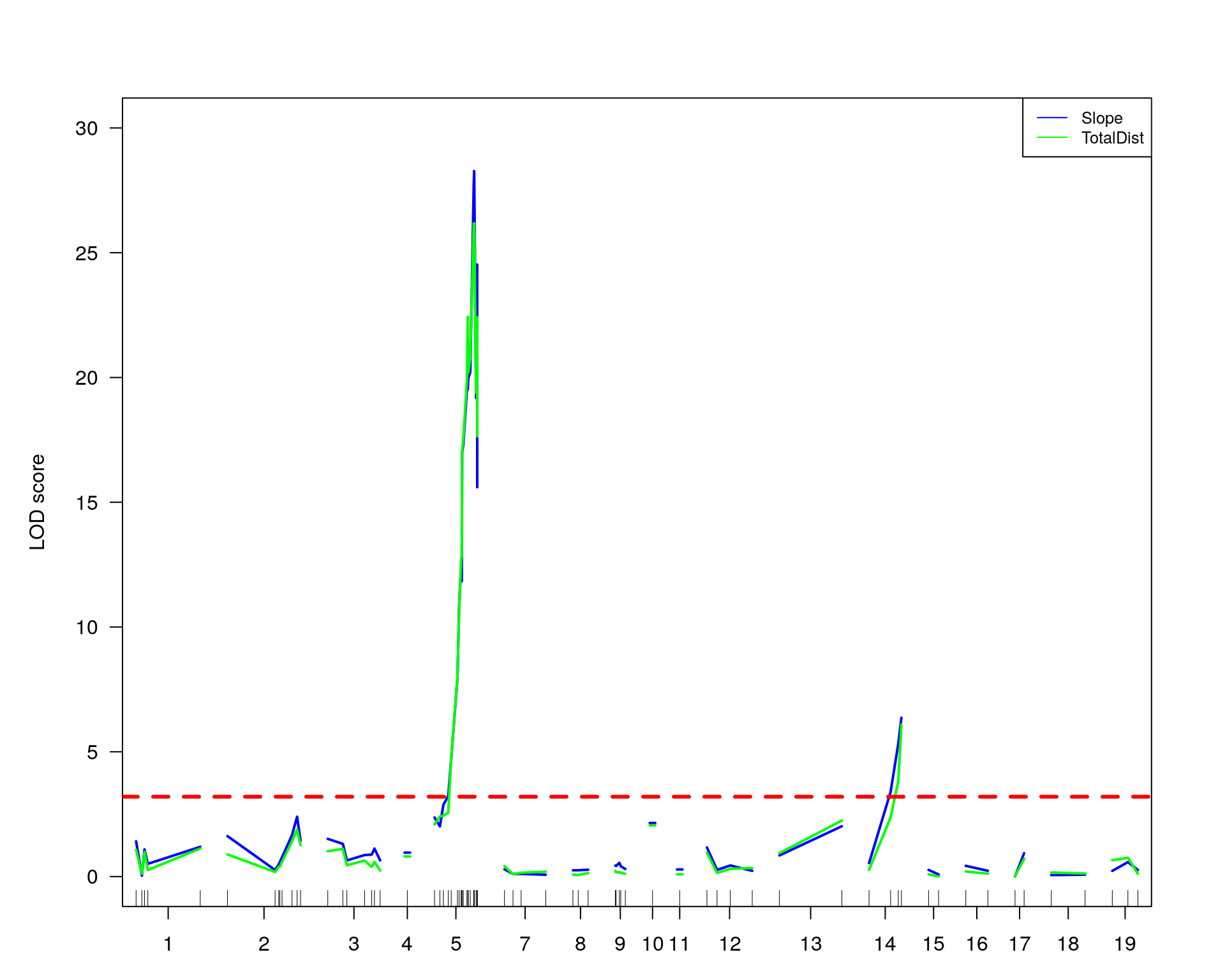
#only at chr 5 and 14
#plot phenotypes: slope and totaldistance3
plot(out.mr[[9]], col= "blue", ylim = c(0, 30), ylab = "LOD score", chr = c(5, 14))
plot(out.mr[[5]], col=  "green", add=TRUE, chr = c(5, 14))
abline(h=3.2, col="red", lty=2, lwd=3)
# Add a legend
legend("topright",
       legend=c("Slope", "TotalDist"),
       col=c("blue", "green"), lty=1, cex=0.8)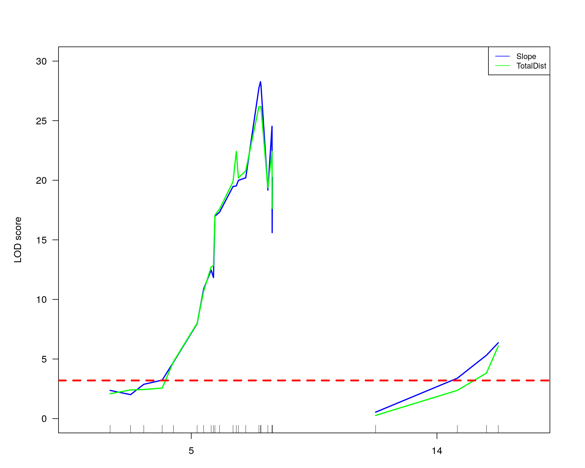
#Interval estimates of the location of QTL are commonly obtained via 1.5-LOD support intervals,
lodint.chr5.slope = lodint(out.mr[[9]], chr= 5)
lodint.chr5.slope
chr pos lod
chr5-133052642-.-T-G 5 72.40547 20.20584
chr5-136332619-.-C-A 5 75.97770 28.27231
chr5-138956439-.-T-C 5 77.76853 19.17899lodint.chr14.slope = lodint(out.mr[[9]], chr= 14)
lodint.chr14.slope chr pos lod
chr14-50642778-.-G-A 14 26.14972 3.390345
chr14-69691477-.-G-T 14 36.07219 6.365103
chr14-69691477-.-G-T 14 36.07219 6.365103lodint.chr5.TotalDist3 = lodint(out.mr[[5]], chr= 5)
lodint.chr5.TotalDist3 chr pos lod
chr5-133052642-.-T-G 5 72.40547 20.78647
chr5-136332619-.-C-A 5 75.97770 26.18011
chr5-136844385-.-T-G 5 76.10078 26.18011
chr5-138956439-.-T-C 5 77.76853 19.37148lodint.chr14.TotalDist3 = lodint(out.mr[[5]], chr= 14)
lodint.chr14.TotalDist3 chr pos lod
chr14-62407765-.-T-A 14 33.20623 3.823005
chr14-69691477-.-G-T 14 36.07219 6.090514
chr14-69691477-.-G-T 14 36.07219 6.090514#genes in the qtl region
# query_variants <- create_variant_query_func("/projects/compsci/vmp/USERS/heh/DO_Opioid/data/cc_variants.sqlite")
# query_genes <- create_gene_query_func("/projects/compsci/vmp/USERS/heh/DO_Opioid/data/mouse_genes_mgi.sqlite")
#
# #the interval for chr5 is 72.40547 to 77.76853 cM, in bp is 133052642 to 138956439
# #Ssc4d at chr5 135.9602 - 135.9745; MGI:MGI:1924709
# chr5_gene <- query_genes(chr = 5, 133.052642, 138.956439)
# plot_genes(chr5_gene)
# #zoom in
# plot_genes(query_genes(5, 135.85, 136.1))
#
# #the interval for chr14 is 26.14972 to 36.07219 cM, in bp is 50642778 to 69691477
# #Kpna3 at chr14 61.36519 - 61.43995; MGI:MGI:1100863
# chr14_gene <- query_genes(chr = 14, 50.642778, 69.691477)
# #zoom in
# plot_genes(query_genes(14, 61.30, 61.50))
#loop for each pheno
for (i in 1:length(idx)){
print(colnames(WT144$pheno)[idx[[i]]])
#save plots
#operm_hist
pdf(paste0("output/", name,"-", colnames(WT144$pheno)[idx[[i]]], ".pdf"), width = 10, height = 10)
plot(operm[[i]][!is.infinite(operm[[i]])], main=paste(name, colnames(WT144$pheno)[idx[[i]]], sep="-"))
#mrscan_pheno
plot(out.mr[[i]], ylab=colnames(WT144$pheno)[idx[[i]]])
add.threshold(out.mr[[i]], perms = operm[[i]], alpha = 0.05, col="magenta")
#pxg
peak = summary(out.mr[[i]], threshold=summary(operm[[i]], alpha = 0.05)[[1]])
print(peak)
marker = c("chr5-136332619-.-C-A", "chr14-69691477-.-G-T")
for (mar in marker){
par(mar=c(3, 5, 4, 3))
plotPXG(WT144, marker=mar, jitter = 0.25, pheno.col = idx[[i]], infer=F, main=paste(mar),
mgp=c(3.4,1,0))
}
#interaction_effect
effectplot(WT144,
mname1 = rownames(peak)[1],
mname2 = rownames(peak)[2],
pheno.col = idx[[i]], add.legend=T, legend.lab = "")
##Multiple-QTL analyses
# After performing the single- and two-QTL genome scans, it’s best to bring the identified loci together into a joint model, which we then refine and from which we may explore the possibility of further QTL. In this effort, we work with “QTL objects” created by makeqtl(). We fit multiple-QTL models with fitqtl(). A number of additional functions will be introduced below.
#First, we create a QTL object containing the loci on chr 5 and 14.
#chr5-136332619-.-C-A 75.97770
#chr14-69691477-.-G-T 36.07219
WT144 <- sim.geno(WT144, n.draws=64)
qtl <- makeqtl(WT144, chr=c(5,14), pos=c(75.97770, 36.07219), what="draws")
out.fq <- fitqtl(WT144, pheno.col=idx[[i]], qtl=qtl, method = "hk")
print(summary(out.fq))
#We may obtain the estimated effects of the QTL via get.ests=TRUE. We use dropone=FALSE to suppress the drop-one-term analysis.
print(summary(fitqtl(WT144, pheno.col=idx[[i]], qtl=qtl, method="hk", get.ests=TRUE, dropone=FALSE)))
#To assess the possibility of an interaction between the two QTL, we may fit the model with the interaction, indicated via a model “formula”.
print("To assess the possibility of an interaction between the two QTL")
out.fqi <- fitqtl(WT144, pheno.col=idx[[i]], qtl=qtl, method="hk", formula=y~Q1+Q2+Q1:Q2)
print(summary(out.fqi))
#complete_scan2
plot(st[[i]])
#toptwo_scan2
plot(st[[i]], chr = summary(out.mr[[i]])[order(-summary(out.mr[[i]])$lod), "chr"][1:2])
dev.off()
}[1] "base.x" chr pos lod
chr5-136332619-.-C-A 5 76.0 11.13
chr14-69691477-.-G-T 14 36.1 4.45
        fitqtl summary

Method: multiple imputation
Model:  normal phenotype
Number of observations : 309

Full model result
----------------------------------
Model formula: y ~ Q1 + Q2

       df           SS         MS     LOD     %var Pvalue(Chi2)  Pvalue(F)
Model   4  12297830859 3074457715 2.29374 3.360698   0.03193929 0.03382928
Error 304 353633004976 1163266464
Total 308 365930835835


Drop one QTL at a time ANOVA table:
----------------------------------
        df Type III SS    LOD   %var F value Pvalue(Chi2) Pvalue(F)
5@76.0   2   9.306e+09 1.7429 2.5432   4.000        0.018    0.0193 *
14@36.1  2   2.545e+09 0.4812 0.6956   1.094        0.330    0.3362
---
Signif. codes:  0 '***' 0.001 '**' 0.01 '*' 0.05 '.' 0.1 ' ' 1


        fitqtl summary

Method: multiple imputation
Model:  normal phenotype
Number of observations : 309

Full model result
----------------------------------
Model formula: y ~ Q1 + Q2

       df           SS         MS     LOD     %var Pvalue(Chi2)  Pvalue(F)
Model   4  12297830859 3074457715 2.29374 3.360698   0.03193929 0.03382928
Error 304 353633004976 1163266464
Total 308 365930835835


Estimated effects:
-----------------
            est    SE      t
Intercept 74119  1978 37.471
5@76.0a   -7492  2719 -2.755
5@76.0d    2176  3947  0.551
14@36.1a  -3581  2982 -1.201
14@36.1d  -2606  3962 -0.658

[1] "To assess the possibility of an interaction between the two QTL"

        fitqtl summary

Method: multiple imputation
Model:  normal phenotype
Number of observations : 309

Full model result
----------------------------------
Model formula: y ~ Q1 + Q2 + Q1:Q2

       df           SS         MS      LOD     %var Pvalue(Chi2)  Pvalue(F)
Model   8  15963802224 1995475278 2.992954 4.362519   0.08759799 0.09532895
Error 300 349967033611 1166556779
Total 308 365930835835


Drop one QTL at a time ANOVA table:
----------------------------------
               df Type III SS    LOD  %var F value Pvalue(Chi2) Pvalue(F)
5@76.0          6   1.297e+10 2.4421 3.545  1.8533        0.081    0.0886 .
14@36.1         6   6.211e+09 1.1804 1.697  0.8874        0.489    0.5044
5@76.0:14@36.1  4   3.666e+09 0.6992 1.002  0.7856        0.522    0.5352
---
Signif. codes:  0 '***' 0.001 '**' 0.01 '*' 0.05 '.' 0.1 ' ' 1
[1] "TestAge.x" chr pos lod
chr5-136332619-.-C-A 5 76.0 21.39
chr14-69691477-.-G-T 14 36.1 5.37
        fitqtl summary

Method: multiple imputation
Model:  normal phenotype
Number of observations : 308

Full model result
----------------------------------
Model formula: y ~ Q1 + Q2

       df        SS         MS      LOD     %var Pvalue(Chi2) Pvalue(F)
Model   4  608750.5 152187.613 25.59048 31.79314            0         0
Error 303 1305972.2   4310.139
Total 307 1914722.7


Drop one QTL at a time ANOVA table:
----------------------------------
        df Type III SS    LOD   %var F value Pvalue(Chi2) Pvalue(F)
5@76.0   2      460710 20.209 24.061   53.44            0   < 2e-16 ***
14@36.1  2       79995  3.976  4.178    9.28            0  0.000123 ***
---
Signif. codes:  0 '***' 0.001 '**' 0.01 '*' 0.05 '.' 0.1 ' ' 1


        fitqtl summary

Method: multiple imputation
Model:  normal phenotype
Number of observations : 308

Full model result
----------------------------------
Model formula: y ~ Q1 + Q2

       df        SS         MS      LOD     %var Pvalue(Chi2) Pvalue(F)
Model   4  608750.5 152187.613 25.59048 31.79314            0         0
Error 303 1305972.2   4310.139
Total 307 1914722.7


Estimated effects:
-----------------
               est       SE        t
Intercept -547.240    3.818 -143.316
5@76.0a     47.751    5.246    9.102
5@76.0d    -35.153    7.592   -4.630
14@36.1a    20.984    5.765    3.640
14@36.1d   -21.954    7.650   -2.870

[1] "To assess the possibility of an interaction between the two QTL"

        fitqtl summary

Method: multiple imputation
Model:  normal phenotype
Number of observations : 308

Full model result
----------------------------------
Model formula: y ~ Q1 + Q2 + Q1:Q2

       df        SS        MS      LOD     %var Pvalue(Chi2) Pvalue(F)
Model   8  719315.2 89914.396 31.50684 37.56759            0         0
Error 299 1195407.5  3998.018
Total 307 1914722.7


Drop one QTL at a time ANOVA table:
----------------------------------
               df Type III SS    LOD   %var F value Pvalue(Chi2) Pvalue(F)
5@76.0          6      571275 26.125 29.836  23.815            0   < 2e-16 ***
14@36.1         6      190560  9.892  9.952   7.944            0  5.84e-08 ***
5@76.0:14@36.1  4      110565  5.916  5.774   6.914            0  2.47e-05 ***
---
Signif. codes:  0 '***' 0.001 '**' 0.01 '*' 0.05 '.' 0.1 ' ' 1
[1] "TotalDist_1" chr pos lod
chr2-137498061-.-T-A 2 67.9 3.38
chr5-136332619-.-C-A 5 76.0 12.52
chr14-62407765-.-T-A 14 33.2 4.48
        fitqtl summary

Method: multiple imputation
Model:  normal phenotype
Number of observations : 309

Full model result
----------------------------------
Model formula: y ~ Q1 + Q2

       df         SS       MS      LOD     %var Pvalue(Chi2)    Pvalue(F)
Model   4  304305506 76076377 14.98858 20.01906 3.641532e-14 5.639933e-14
Error 304 1215773537  3999255
Total 308 1520079043


Drop one QTL at a time ANOVA table:
----------------------------------
        df Type III SS    LOD   %var F value Pvalue(Chi2) Pvalue(F)
5@76.0   2   211918140 10.781 13.941  26.495        0.000  2.47e-11 ***
14@36.1  2    58257987  3.141  3.833   7.284        0.001  0.000813 ***
---
Signif. codes:  0 '***' 0.001 '**' 0.01 '*' 0.05 '.' 0.1 ' ' 1


        fitqtl summary

Method: multiple imputation
Model:  normal phenotype
Number of observations : 309

Full model result
----------------------------------
Model formula: y ~ Q1 + Q2

       df         SS       MS      LOD     %var Pvalue(Chi2)    Pvalue(F)
Model   4  304305506 76076377 14.98858 20.01906 3.641532e-14 5.639933e-14
Error 304 1215773537  3999255
Total 308 1520079043


Estimated effects:
-----------------
              est      SE      t
Intercept 8572.85  116.00 73.904
5@76.0a    962.91  159.33  6.044
5@76.0d   -892.25  231.12 -3.860
14@36.1a   648.40  174.86  3.708
14@36.1d    67.83  232.37  0.292

[1] "To assess the possibility of an interaction between the two QTL"

        fitqtl summary

Method: multiple imputation
Model:  normal phenotype
Number of observations : 309

Full model result
----------------------------------
Model formula: y ~ Q1 + Q2 + Q1:Q2

       df         SS       MS      LOD     %var Pvalue(Chi2)    Pvalue(F)
Model   8  310866295 38858287 15.35165 20.45067 3.569922e-12 6.744161e-12
Error 300 1209212748  4030709
Total 308 1520079043


Drop one QTL at a time ANOVA table:
----------------------------------
               df Type III SS     LOD    %var F value Pvalue(Chi2) Pvalue(F)
5@76.0          6   218478928 11.1443 14.3729  9.0339        0.000  4.38e-09
14@36.1         6    64818775  3.5037  4.2642  2.6802        0.013    0.0151
5@76.0:14@36.1  4     6560788  0.3631  0.4316  0.4069        0.796    0.8036

5@76.0         ***
14@36.1        *
5@76.0:14@36.1
---
Signif. codes:  0 '***' 0.001 '**' 0.01 '*' 0.05 '.' 0.1 ' ' 1
[1] "TotalDist_2" chr pos lod
chr2-137498061-.-T-A 2 67.9 3.60
chr5-136332619-.-C-A 5 76.0 24.45
chr14-69691477-.-G-T 14 36.1 4.61
        fitqtl summary

Method: multiple imputation
Model:  normal phenotype
Number of observations : 308

Full model result
----------------------------------
Model formula: y ~ Q1 + Q2

       df         SS        MS      LOD     %var Pvalue(Chi2) Pvalue(F)
Model   4 1416757547 354189387 26.93466 33.15027            0         0
Error 303 2856985472   9428995
Total 307 4273743020


Drop one QTL at a time ANOVA table:
----------------------------------
        df Type III SS    LOD   %var F value Pvalue(Chi2) Pvalue(F)
5@76.0   2   1.134e+09 22.363 26.544  60.155        0.000   < 2e-16 ***
14@36.1  2   1.434e+08  3.276  3.356   7.606        0.001  0.000599 ***
---
Signif. codes:  0 '***' 0.001 '**' 0.01 '*' 0.05 '.' 0.1 ' ' 1


        fitqtl summary

Method: multiple imputation
Model:  normal phenotype
Number of observations : 308

Full model result
----------------------------------
Model formula: y ~ Q1 + Q2

       df         SS        MS      LOD     %var Pvalue(Chi2) Pvalue(F)
Model   4 1416757547 354189387 26.93466 33.15027            0         0
Error 303 2856985472   9428995
Total 307 4273743020


Estimated effects:
-----------------
              est      SE      t
Intercept  7248.7   178.6 40.589
5@76.0a    2302.6   245.2  9.391
5@76.0d   -1911.3   355.1 -5.382
14@36.1a   1048.0   269.7  3.886
14@36.1d   -347.7   357.7 -0.972

[1] "To assess the possibility of an interaction between the two QTL"

        fitqtl summary

Method: multiple imputation
Model:  normal phenotype
Number of observations : 308

Full model result
----------------------------------
Model formula: y ~ Q1 + Q2 + Q1:Q2

       df         SS        MS    LOD     %var Pvalue(Chi2) Pvalue(F)
Model   8 1497747285 187218411 28.858 35.04533            0         0
Error 299 2775995735   9284267
Total 307 4273743020


Drop one QTL at a time ANOVA table:
----------------------------------
               df Type III SS    LOD   %var F value Pvalue(Chi2) Pvalue(F)
5@76.0          6   1.215e+09 24.287 28.439  21.818        0.000   < 2e-16 ***
14@36.1         6   2.244e+08  5.199  5.251   4.029        0.001  0.000673 ***
5@76.0:14@36.1  4   8.099e+07  1.923  1.895   2.181        0.065  0.071126 .
---
Signif. codes:  0 '***' 0.001 '**' 0.01 '*' 0.05 '.' 0.1 ' ' 1
[1] "TotalDist_3" chr pos lod
chr5-136332619-.-C-A 5 76.0 26.18
chr14-69691477-.-G-T 14 36.1 6.09
        fitqtl summary

Method: multiple imputation
Model:  normal phenotype
Number of observations : 281

Full model result
----------------------------------
Model formula: y ~ Q1 + Q2

       df         SS        MS      LOD     %var Pvalue(Chi2) Pvalue(F)
Model   4 3170972617 792743154 31.45631 40.28112            0         0
Error 276 4701133507  17033092
Total 280 7872106124


Drop one QTL at a time ANOVA table:
----------------------------------
        df Type III SS    LOD   %var F value Pvalue(Chi2) Pvalue(F)
5@76.0   2   2.423e+09 25.367 30.783   71.13            0   < 2e-16 ***
14@36.1  2   4.478e+08  5.552  5.689   13.15            0  3.52e-06 ***
---
Signif. codes:  0 '***' 0.001 '**' 0.01 '*' 0.05 '.' 0.1 ' ' 1


        fitqtl summary

Method: multiple imputation
Model:  normal phenotype
Number of observations : 281

Full model result
----------------------------------
Model formula: y ~ Q1 + Q2

       df         SS        MS      LOD     %var Pvalue(Chi2) Pvalue(F)
Model   4 3170972617 792743154 31.45631 40.28112            0         0
Error 276 4701133507  17033092
Total 280 7872106124


Estimated effects:
-----------------
              est      SE      t
Intercept  7106.2   251.6 28.249
5@76.0a    3548.9   349.2 10.162
5@76.0d   -2908.4   497.5 -5.846
14@36.1a   1818.8   380.1  4.785
14@36.1d  -1335.6   503.4 -2.653

[1] "To assess the possibility of an interaction between the two QTL"

        fitqtl summary

Method: multiple imputation
Model:  normal phenotype
Number of observations : 281

Full model result
----------------------------------
Model formula: y ~ Q1 + Q2 + Q1:Q2

       df         SS        MS      LOD     %var Pvalue(Chi2) Pvalue(F)
Model   8 3558447363 444805920 36.70494 45.20324            0         0
Error 272 4313658761  15859040
Total 280 7872106124


Drop one QTL at a time ANOVA table:
----------------------------------
               df Type III SS    LOD   %var F value Pvalue(Chi2) Pvalue(F)
5@76.0          6   2.811e+09 30.615 35.705  29.539            0   < 2e-16 ***
14@36.1         6   8.353e+08 10.801 10.611   8.778            0  9.41e-09 ***
5@76.0:14@36.1  4   3.875e+08  5.249  4.922   6.108            0  0.000101 ***
---
Signif. codes:  0 '***' 0.001 '**' 0.01 '*' 0.05 '.' 0.1 ' ' 1
[1] "base.y" chr pos lod
chr5-136332619-.-C-A 5 76.0 11.20
chr14-69691477-.-G-T 14 36.1 3.38
        fitqtl summary

Method: multiple imputation
Model:  normal phenotype
Number of observations : 307

Full model result
----------------------------------
Model formula: y ~ Q1 + Q2

       df          SS        MS      LOD     %var Pvalue(Chi2)    Pvalue(F)
Model   4  2305025387 576256347 9.408325 13.16237 8.851194e-09 1.160207e-08
Error 302 15207217015  50355023
Total 306 17512242403


Drop one QTL at a time ANOVA table:
----------------------------------
        df Type III SS   LOD   %var F value Pvalue(Chi2) Pvalue(F)
5@76.0   2   1.850e+09 7.652 10.562   18.37         0.00  2.97e-08 ***
14@36.1  2   2.206e+08 0.960  1.259    2.19         0.11     0.114
---
Signif. codes:  0 '***' 0.001 '**' 0.01 '*' 0.05 '.' 0.1 ' ' 1


        fitqtl summary

Method: multiple imputation
Model:  normal phenotype
Number of observations : 307

Full model result
----------------------------------
Model formula: y ~ Q1 + Q2

       df          SS        MS      LOD     %var Pvalue(Chi2)    Pvalue(F)
Model   4  2305025387 576256347 9.408325 13.16237 8.851194e-09 1.160207e-08
Error 302 15207217015  50355023
Total 306 17512242403


Estimated effects:
-----------------
              est      SE       t
Intercept -5438.5   412.5 -13.185
5@76.0a   -3189.4   569.8  -5.598
5@76.0d    1762.9   824.0   2.139
14@36.1a  -1158.0   622.3  -1.861
14@36.1d   1023.2   827.4   1.237

[1] "To assess the possibility of an interaction between the two QTL"

        fitqtl summary

Method: multiple imputation
Model:  normal phenotype
Number of observations : 307

Full model result
----------------------------------
Model formula: y ~ Q1 + Q2 + Q1:Q2

       df          SS        MS      LOD     %var Pvalue(Chi2)    Pvalue(F)
Model   8  2838790053 354848757 11.79025 16.21032 6.048155e-09 9.752631e-09
Error 298 14673452350  49239773
Total 306 17512242403


Drop one QTL at a time ANOVA table:
----------------------------------
               df Type III SS    LOD   %var F value Pvalue(Chi2) Pvalue(F)
5@76.0          6   2.383e+09 10.034 13.610   8.067        0.000  4.37e-08 ***
14@36.1         6   7.543e+08  3.342  4.307   2.553        0.017    0.0200 *
5@76.0:14@36.1  4   5.338e+08  2.382  3.048   2.710        0.027    0.0304 *
---
Signif. codes:  0 '***' 0.001 '**' 0.01 '*' 0.05 '.' 0.1 ' ' 1
[1] "TestAge.y" chr pos lod
chr5-136332619-.-C-A 5 76.0 21.31
chr14-69691477-.-G-T 14 36.1 5.34
        fitqtl summary

Method: multiple imputation
Model:  normal phenotype
Number of observations : 307

Full model result
----------------------------------
Model formula: y ~ Q1 + Q2

       df      SS         MS      LOD     %var Pvalue(Chi2) Pvalue(F)
Model   4  608148 152037.000 25.48688 31.77214            0         0
Error 302 1305944   4324.317
Total 306 1914092


Drop one QTL at a time ANOVA table:
----------------------------------
        df Type III SS    LOD   %var F value Pvalue(Chi2) Pvalue(F)
5@76.0   2      460487 20.135 24.058   53.24            0   < 2e-16 ***
14@36.1  2       80085  3.968  4.184    9.26            0  0.000125 ***
---
Signif. codes:  0 '***' 0.001 '**' 0.01 '*' 0.05 '.' 0.1 ' ' 1


        fitqtl summary

Method: multiple imputation
Model:  normal phenotype
Number of observations : 307

Full model result
----------------------------------
Model formula: y ~ Q1 + Q2

       df      SS         MS      LOD     %var Pvalue(Chi2) Pvalue(F)
Model   4  608148 152037.000 25.48688 31.77214            0         0
Error 302 1305944   4324.317
Total 306 1914092


Estimated effects:
-----------------
              est      SE      t
Intercept  26.175   3.830  6.835
5@76.0a    47.817   5.273  9.068
5@76.0d   -35.018   7.624 -4.593
14@36.1a   21.080   5.790  3.641
14@36.1d  -21.902   7.674 -2.854

[1] "To assess the possibility of an interaction between the two QTL"

        fitqtl summary

Method: multiple imputation
Model:  normal phenotype
Number of observations : 307

Full model result
----------------------------------
Model formula: y ~ Q1 + Q2 + Q1:Q2

       df        SS        MS      LOD     %var Pvalue(Chi2) Pvalue(F)
Model   8  718710.4 89838.804 31.38404 37.54838            0         0
Error 298 1195381.3  4011.347
Total 306 1914091.7


Drop one QTL at a time ANOVA table:
----------------------------------
               df Type III SS    LOD   %var F value Pvalue(Chi2) Pvalue(F)
5@76.0          6      571049 26.032 29.834  23.726            0   < 2e-16 ***
14@36.1         6      190647  9.865  9.960   7.921            0  6.19e-08 ***
5@76.0:14@36.1  4      110562  5.897  5.776   6.891            0  2.57e-05 ***
---
Signif. codes:  0 '***' 0.001 '**' 0.01 '*' 0.05 '.' 0.1 ' ' 1
[1] "Intercept" chr pos lod
chr5-136332619-.-C-A 5 76.0 27.06
chr14-69691477-.-G-T 14 36.1 6.12
        fitqtl summary

Method: multiple imputation
Model:  normal phenotype
Number of observations : 309

Full model result
----------------------------------
Model formula: y ~ Q1 + Q2

       df         SS        MS      LOD     %var Pvalue(Chi2) Pvalue(F)
Model   4 1075780655 268945164 31.46456 37.43292            0         0
Error 304 1798108751   5914831
Total 308 2873889406


Drop one QTL at a time ANOVA table:
----------------------------------
        df Type III SS    LOD   %var F value Pvalue(Chi2) Pvalue(F)
5@76.0   2   824088260 25.315 28.675   69.66            0   < 2e-16 ***
14@36.1  2   125918689  4.542  4.381   10.64            0   3.4e-05 ***
---
Signif. codes:  0 '***' 0.001 '**' 0.01 '*' 0.05 '.' 0.1 ' ' 1


        fitqtl summary

Method: multiple imputation
Model:  normal phenotype
Number of observations : 309

Full model result
----------------------------------
Model formula: y ~ Q1 + Q2

       df         SS        MS      LOD     %var Pvalue(Chi2) Pvalue(F)
Model   4 1075780655 268945164 31.46456 37.43292            0         0
Error 304 1798108751   5914831
Total 308 2873889406


Estimated effects:
-----------------
              est      SE       t
Intercept 10313.5   141.1  73.091
5@76.0a   -1974.0   193.9 -10.182
5@76.0d    1583.6   281.1   5.634
14@36.1a   -918.0   212.7  -4.316
14@36.1d    651.9   282.7   2.306

[1] "To assess the possibility of an interaction between the two QTL"

        fitqtl summary

Method: multiple imputation
Model:  normal phenotype
Number of observations : 309

Full model result
----------------------------------
Model formula: y ~ Q1 + Q2 + Q1:Q2

       df         SS        MS      LOD     %var Pvalue(Chi2) Pvalue(F)
Model   8 1201400132 150175016 36.32399 41.80398            0         0
Error 300 1672489274   5574964
Total 308 2873889406


Drop one QTL at a time ANOVA table:
----------------------------------
               df Type III SS    LOD   %var F value Pvalue(Chi2) Pvalue(F)
5@76.0          6   949707736 30.174 33.046  28.392            0   < 2e-16 ***
14@36.1         6   251538166  9.401  8.753   7.520            0   1.6e-07 ***
5@76.0:14@36.1  4   125619476  4.859  4.371   5.633            0   0.00022 ***
---
Signif. codes:  0 '***' 0.001 '**' 0.01 '*' 0.05 '.' 0.1 ' ' 1
[1] "Slope" chr pos lod
chr5-136332619-.-C-A 5 76.0 28.27
chr14-69691477-.-G-T 14 36.1 6.37
        fitqtl summary

Method: multiple imputation
Model:  normal phenotype
Number of observations : 309

Full model result
----------------------------------
Model formula: y ~ Q1 + Q2

       df        SS         MS      LOD     %var Pvalue(Chi2) Pvalue(F)
Model   4  464743.5 116185.868 32.77441 38.64247            0         0
Error 304  737932.0   2427.408
Total 308 1202675.5


Drop one QTL at a time ANOVA table:
----------------------------------
        df Type III SS   LOD  %var F value Pvalue(Chi2) Pvalue(F)
5@76.0   2      355562 26.39 29.56   73.24            0   < 2e-16 ***
14@36.1  2       55199  4.84  4.59   11.37            0  1.73e-05 ***
---
Signif. codes:  0 '***' 0.001 '**' 0.01 '*' 0.05 '.' 0.1 ' ' 1


        fitqtl summary

Method: multiple imputation
Model:  normal phenotype
Number of observations : 309

Full model result
----------------------------------
Model formula: y ~ Q1 + Q2

       df        SS         MS      LOD     %var Pvalue(Chi2) Pvalue(F)
Model   4  464743.5 116185.868 32.77441 38.64247            0         0
Error 304  737932.0   2427.408
Total 308 1202675.5


Estimated effects:
-----------------
              est      SE      t
Intercept -26.054   2.858 -9.116
5@76.0a    40.819   3.925 10.400
5@76.0d   -33.287   5.694 -5.846
14@36.1a   19.768   4.308  4.589
14@36.1d  -11.565   5.725 -2.020

[1] "To assess the possibility of an interaction between the two QTL"

        fitqtl summary

Method: multiple imputation
Model:  normal phenotype
Number of observations : 309

Full model result
----------------------------------
Model formula: y ~ Q1 + Q2 + Q1:Q2

       df        SS        MS      LOD     %var Pvalue(Chi2) Pvalue(F)
Model   8  507355.4 63419.425 36.76539 42.18556            0         0
Error 300  695320.1  2317.734
Total 308 1202675.5


Drop one QTL at a time ANOVA table:
----------------------------------
               df Type III SS    LOD   %var F value Pvalue(Chi2) Pvalue(F)
5@76.0          6      398174 30.380 33.107  28.632        0.000   < 2e-16 ***
14@36.1         6       97810  8.831  8.133   7.033        0.000  5.11e-07 ***
5@76.0:14@36.1  4       42612  3.991  3.543   4.596        0.001   0.00129 **
---
Signif. codes:  0 '***' 0.001 '**' 0.01 '*' 0.05 '.' 0.1 ' ' 1
Plot the Dist_vs_age separate by genotype for each marker
plot_graph <- function(cross, name){
  # Plot the Dist vs age, separate by genotype for each marker
  allphen <- cross$pheno
  allgeno <- as.data.frame(pull.geno(cross))
  rownames(allgeno) <- cross$pheno$AnimalName
  allphen <- merge(allphen, allgeno, by.x="AnimalName", by.y="row.names", all.x=TRUE)
  pdf(paste0("output/", name, "_TotalDist_vs_TestAge_by_marker.pdf"))
  for (mar in colnames(allgeno)){
    subplot <- allphen[!is.na(allphen[,mar, drop=FALSE]),] %>%
      pivot_longer(cols = starts_with("TestAge_"), names_to="test.no", values_to = "Age") %>%
      separate(test.no, c("empty1", "test1")) %>%
      pivot_longer(cols = starts_with("TotalDist_"), names_to="test.no.2", values_to = "Dist") %>%
      separate(test.no.2, c("empty2", "test2")) %>% filter(test1==test2)
    subplot <- as.data.frame(subplot)
    subplot[, mar] <- factor(subplot[, mar, drop=T])
    levels(subplot[,mar]) <- c("AA","AB","BB")
    p <- ggplot(subplot, aes(Age, Dist, color=get(mar), group=get(mar))) +
      geom_point() +
      labs(color = "Genotype") +
      scale_color_brewer(palette = "Set1") +
      stat_smooth(method="lm", show.legend = FALSE, formula = y~x) +
      labs(title=paste0("effect for marker ", mar))
    print(p)
  }
  dev.off()
}

plot_int_graph <- function(cross, name,  basem){
  # Plot the Dist vs age, separate by genotype for each marker
  allphen <- cross$pheno
  allgeno <- as.data.frame(pull.geno(cross))
  rownames(allgeno) <- cross$pheno$AnimalName
  allphen <- merge(allphen, allgeno, by.x="AnimalName", by.y="row.names", all.x=TRUE)
  #pdf(paste0("output/", name, ".pdf"))
  for (mar in colnames(allgeno)){
    print(mar)
    subplot <- allphen[!is.na(allphen[,mar, drop=FALSE]),] %>%
      pivot_longer(cols = starts_with("TestAge_"), names_to="test.no", values_to = "Age") %>%
      separate(test.no, c("empty1", "test1")) %>%
      pivot_longer(cols = starts_with("TotalDist_"), names_to="test.no.2", values_to = "Dist") %>%
      separate(test.no.2, c("empty2", "test2")) %>% filter(test1==test2)
    subplot <- as.data.frame(subplot)
    subplot$interactions <- factor(subplot[, basem] + subplot[, mar]*3)
    # 1:1 -> 4 1:2 -> 7 1:3 -> 10
    # 2:1 -> 5 2:2 -> 8 2:3 -> 11
    # 3:1 -> 6 3:2 -> 9 3:3 -> 12
    itypes  <- c(1,2,3,"AA:AA", "AB:AA", "BB:AA",
                "AA:AB", "AB:AB", "BB:AB",
                "AA:BB", "AB:BB", "BB:BB")
    levels(subplot$interactions) <- itypes[as.integer(levels(subplot$interactions))]

    #replaces 1 2 and 3 as AA, AB and BB
    subplot[, basem][subplot[, basem] == 1] <- "AA"
    subplot[, basem][subplot[, basem] == 2] <- "AB"
    subplot[, basem][subplot[, basem] == 3] <- "BB"
    subplot[, mar][subplot[, mar] == 1] <- "AA"
    subplot[, mar][subplot[, mar] == 2] <- "AB"
    subplot[, mar][subplot[, mar] == 3] <- "BB"

    p1 <- ggplot(subplot, aes(Age, Dist, color=interactions, group=interactions)) +
      geom_point(shape = 20) +
      #scale_color_discrete("Genotype") +
      labs(color = "Genotype") +
      ylab("TotalDist") +
      xlab("TestAge") +
      #scale_color_brewer(palette = "Set1") +
      scale_color_manual(breaks = c("AA:AA", "AB:AA", "BB:AA", "AA:AB",
                                    "AB:AB", "BB:AB", "AA:BB", "AB:BB", "BB:BB"),
                                         #values = RColorBrewer::brewer.pal(9, "Set1")[9:1]) +
                       values = c("#999999", "#F781BF", "#A65628","#9a9a00", "#FF7F00", "#984EA3", "#4DAF4A", "#377EB8", "#E41A1C")) +
      stat_smooth(method="lm", show.legend = FALSE, formula = y~x) +
      labs(title=paste0("effect for markers ", basem, " x ", mar)) +
      theme_bw()
    print(p1)

    p2 <- ggplot(subplot, aes(Age, Dist, color=interactions, group=interactions)) +
      geom_point(shape = 20) +
      geom_line(aes(group = AnimalName, color = interactions), show.legend = FALSE, alpha = 0.2) +
      geom_smooth(method='lm', formula= y~x, show.legend = FALSE) +
      #scale_color_discrete("Genotype") +
      labs(color = "Genotype") +
      ylab("TotalDist") +
      xlab("TestAge") +
      #scale_color_brewer(palette = "Set1") +
      scale_color_manual(breaks = c("AA:AA", "AB:AA", "BB:AA", "AA:AB",
                                    "AB:AB", "BB:AB", "AA:BB", "AB:BB", "BB:BB"),
                                         #values = RColorBrewer::brewer.pal(9, "Set1")[9:1]) +
                       values = c("#999999", "#F781BF", "#A65628","#9a9a00", "#FF7F00", "#984EA3", "#4DAF4A", "#377EB8", "#E41A1C")) +
      stat_smooth(method="lm", show.legend = FALSE, formula = y~x) +
      labs(title=paste0("Effect for markers ", basem, " x ", mar)) +
      facet_grid(subplot[, basem] ~ subplot[, mar]) +
      theme_bw() +
      theme(plot.title = element_text(size=6))
    print(p2)
  }
  #dev.off()
}
plot_graph(WT144, "WT144_effect_for_marker_plots")
png
2 plot_int_graph(WT144, paste0("WT144_effect_for_marker_", "_int_chr5-136332619-.-C-A"), "chr5-136332619-.-C-A")[1] "chr1-65643621-.-C-A"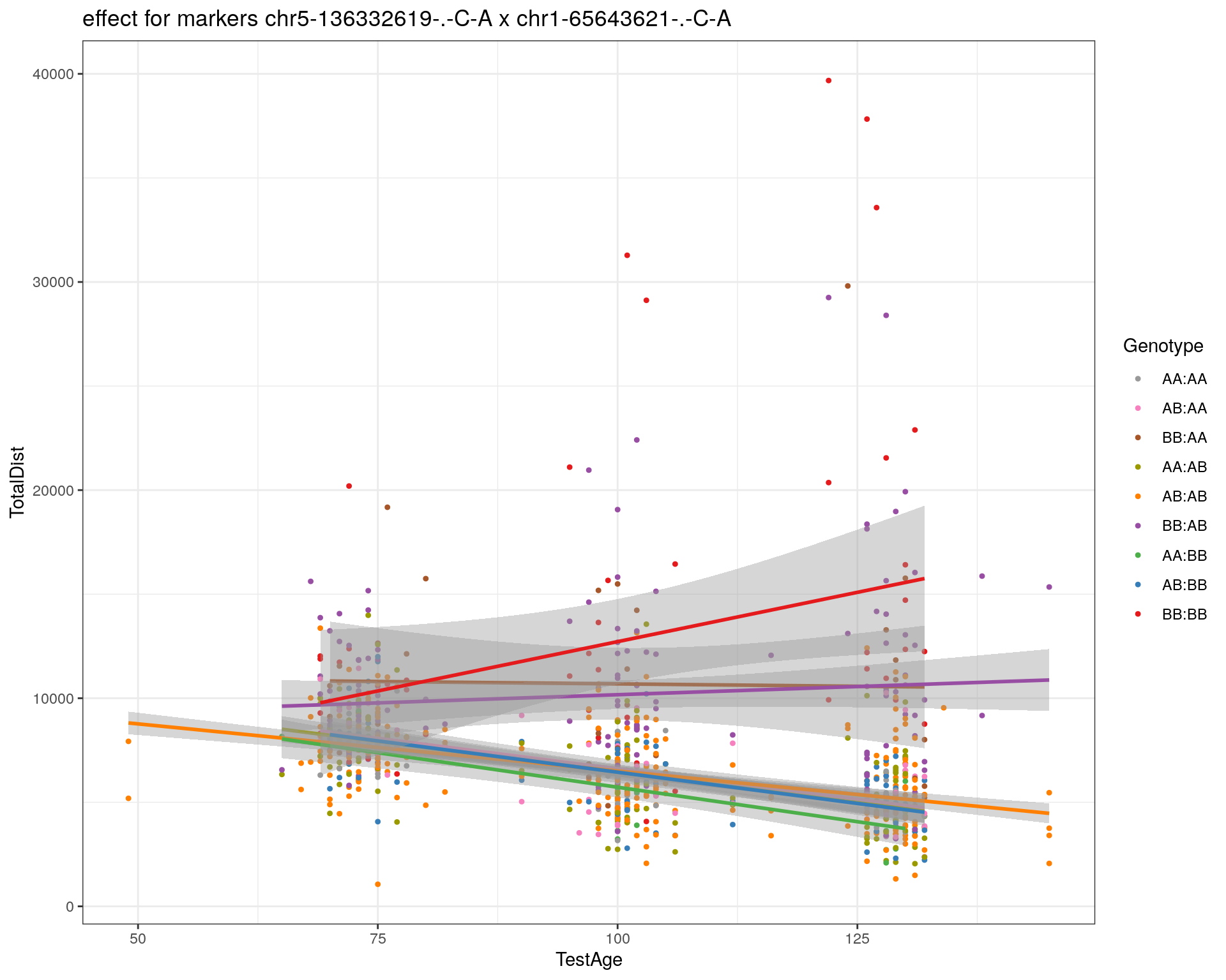

[1] "chr1-74679418-.-A-G"
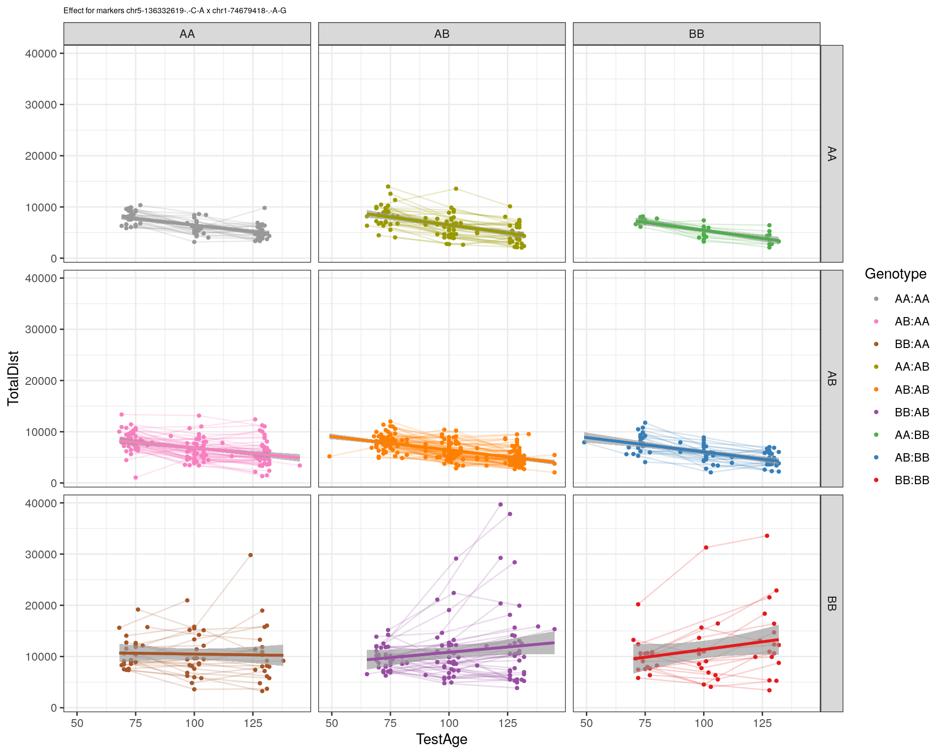
[1] "chr1-79823528-.-A-G"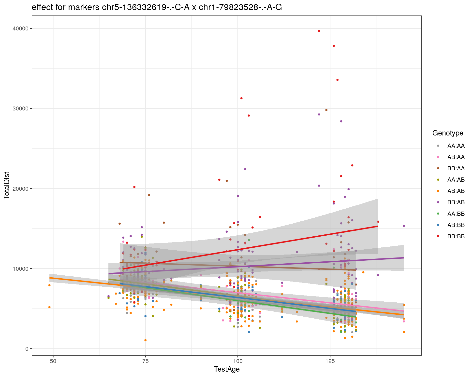
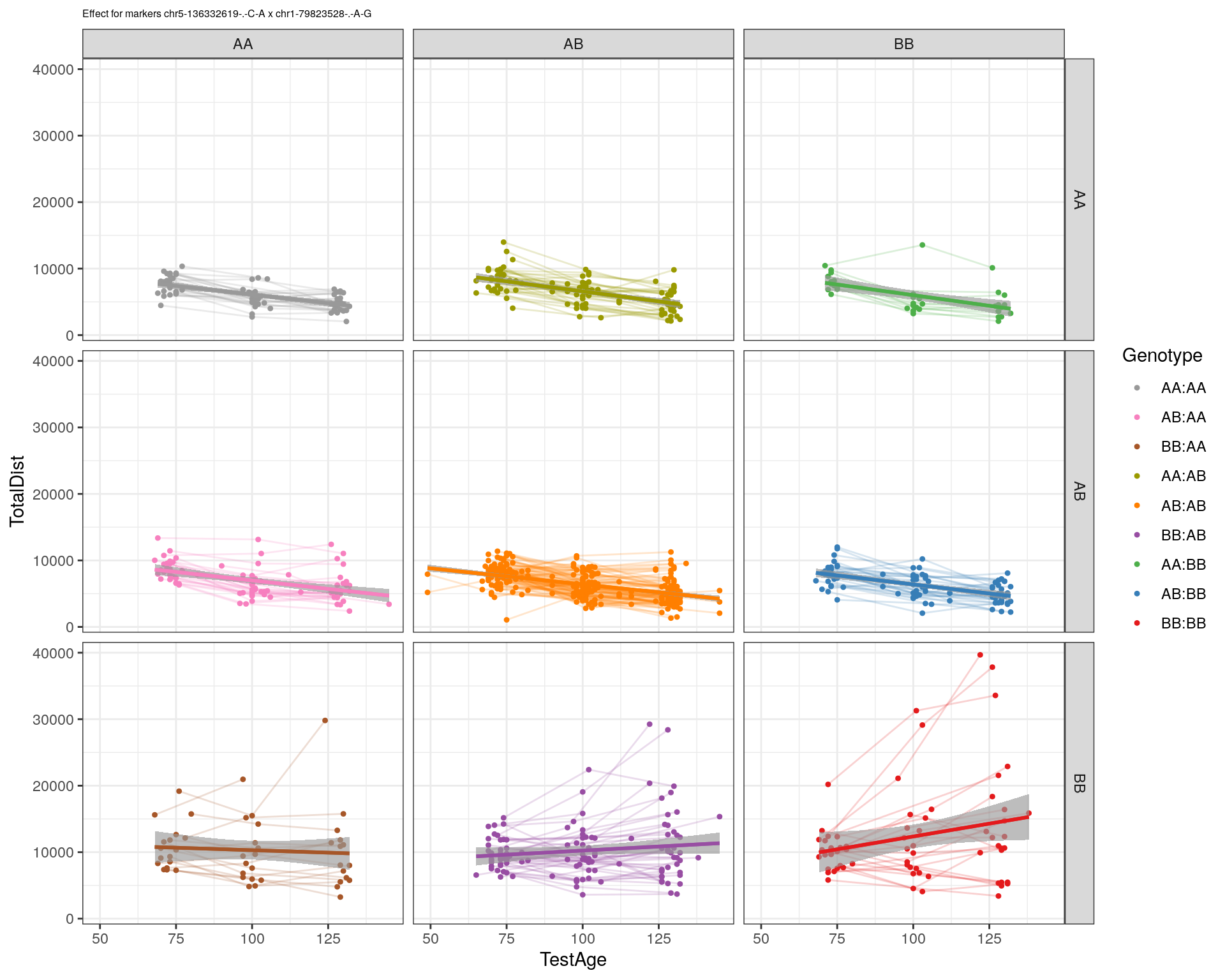
[1] "chr1-86851039-.-A-G"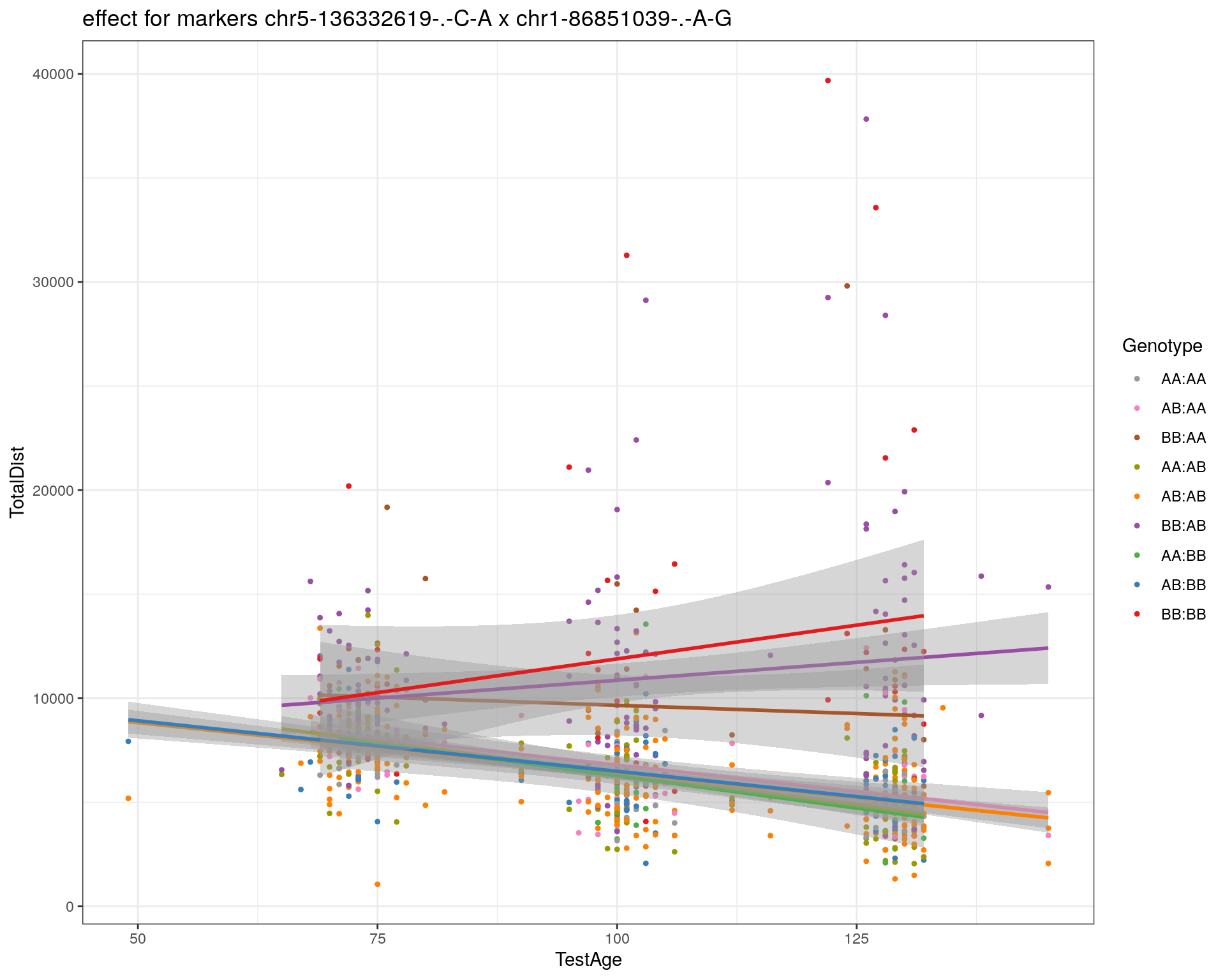
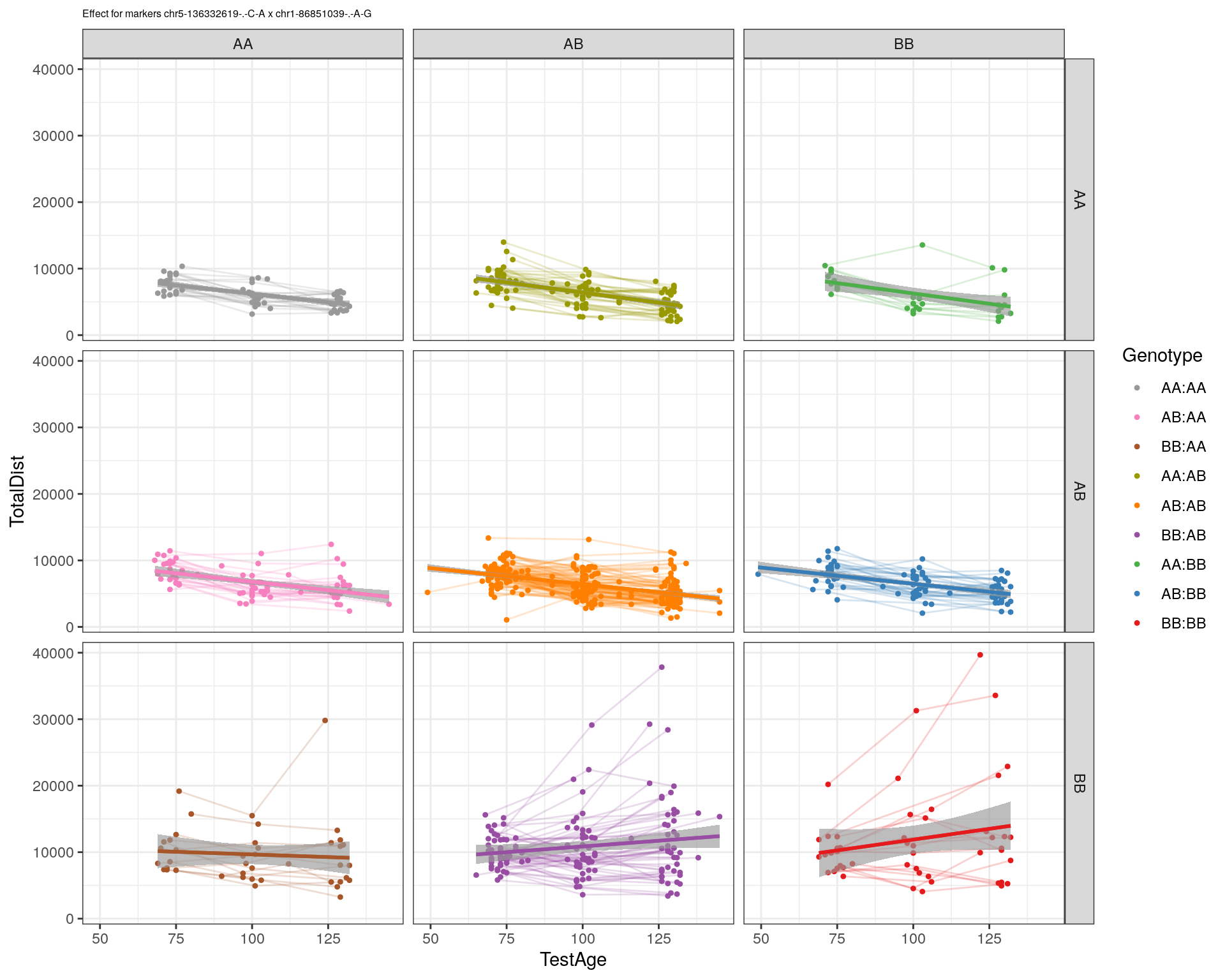
[1] "chr1-188155143-.-G-A"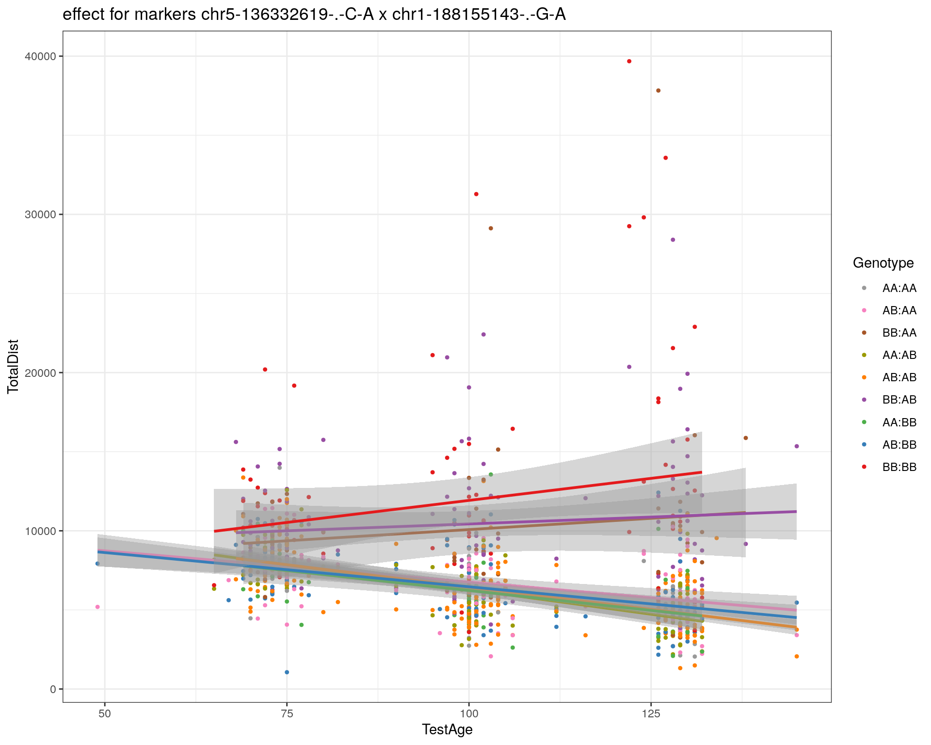
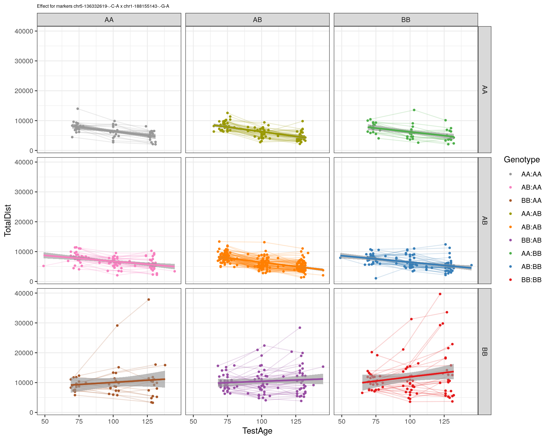
[1] "chr2-7018694-.-G-T"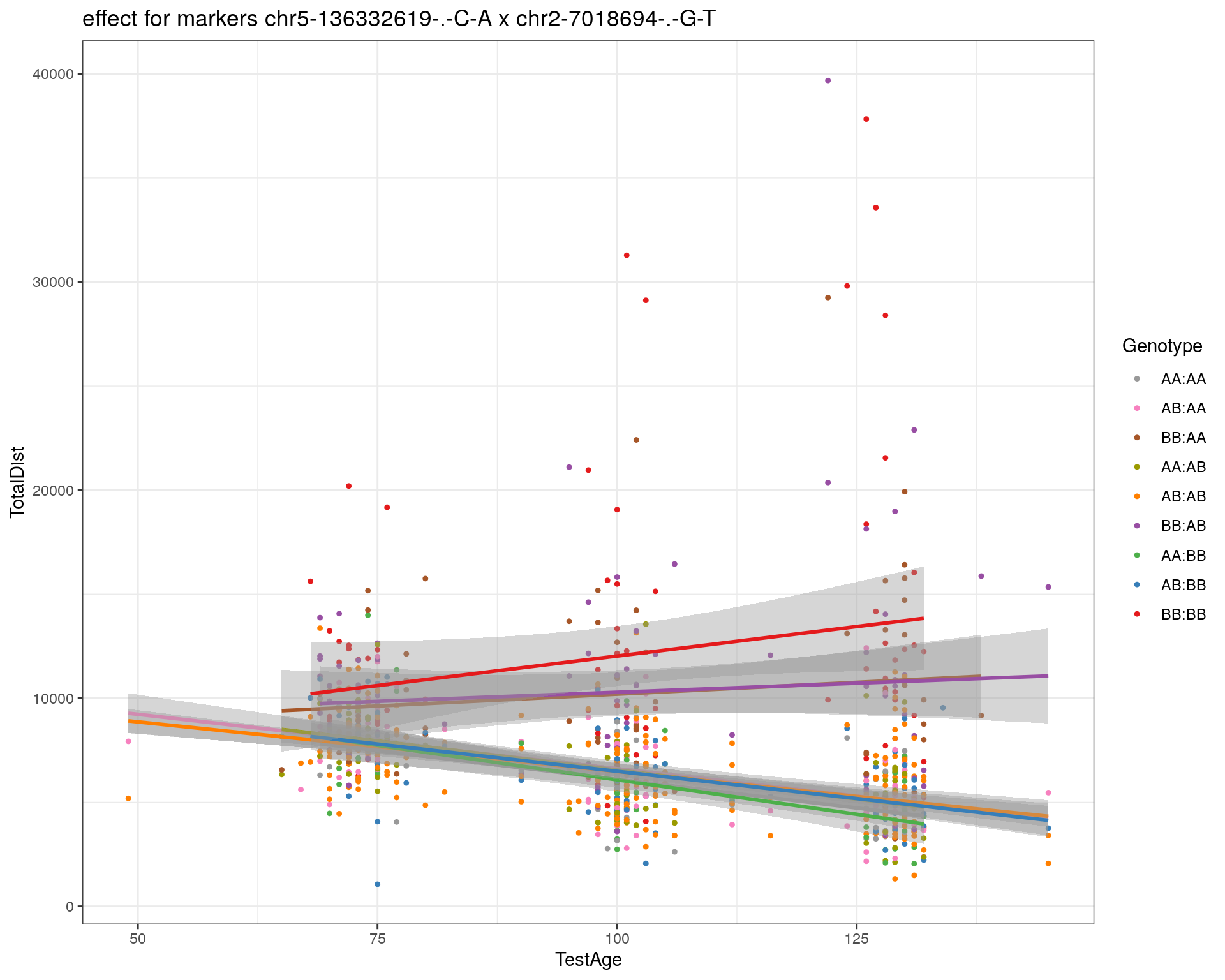
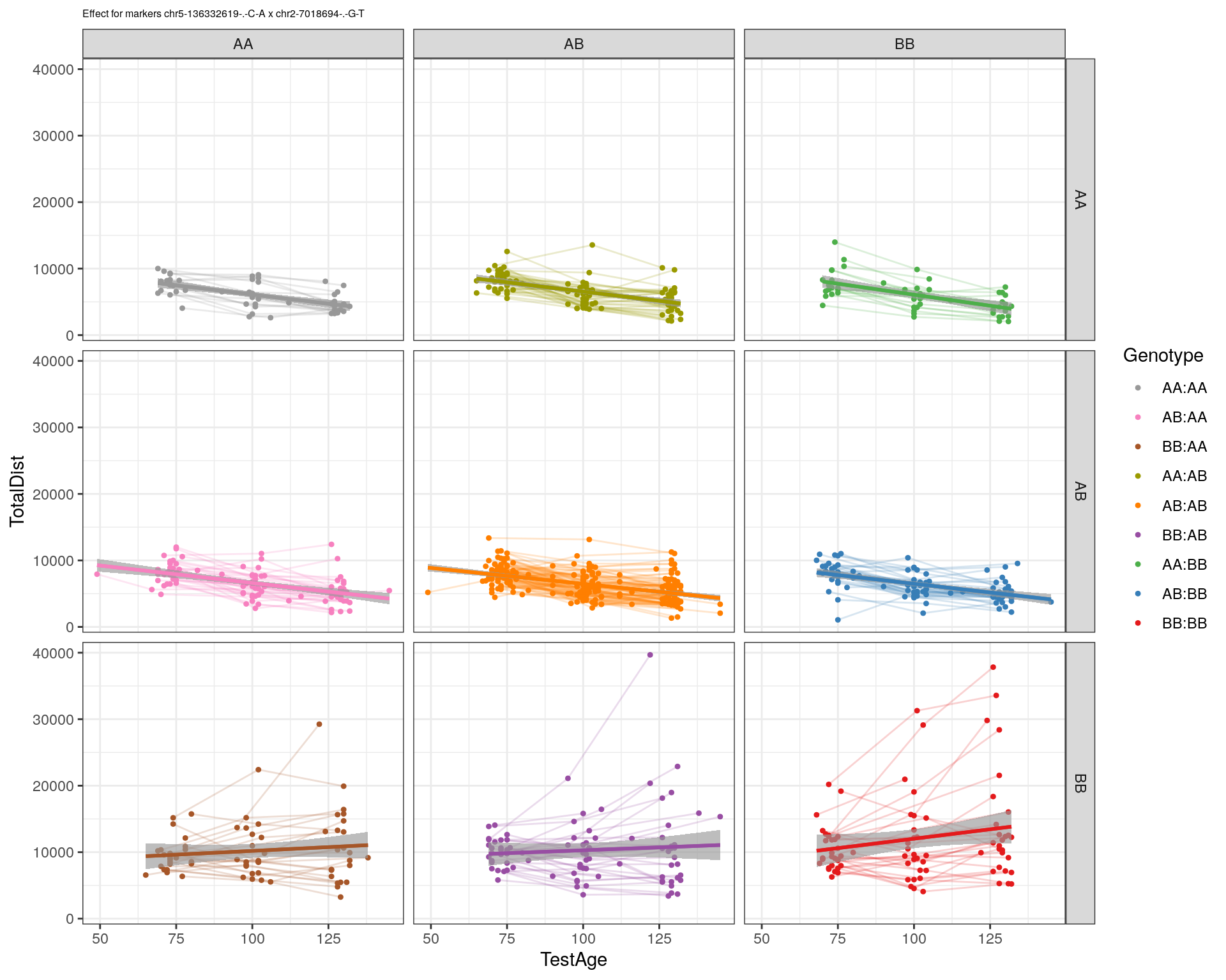
[1] "chr2-79706301-.-T-A"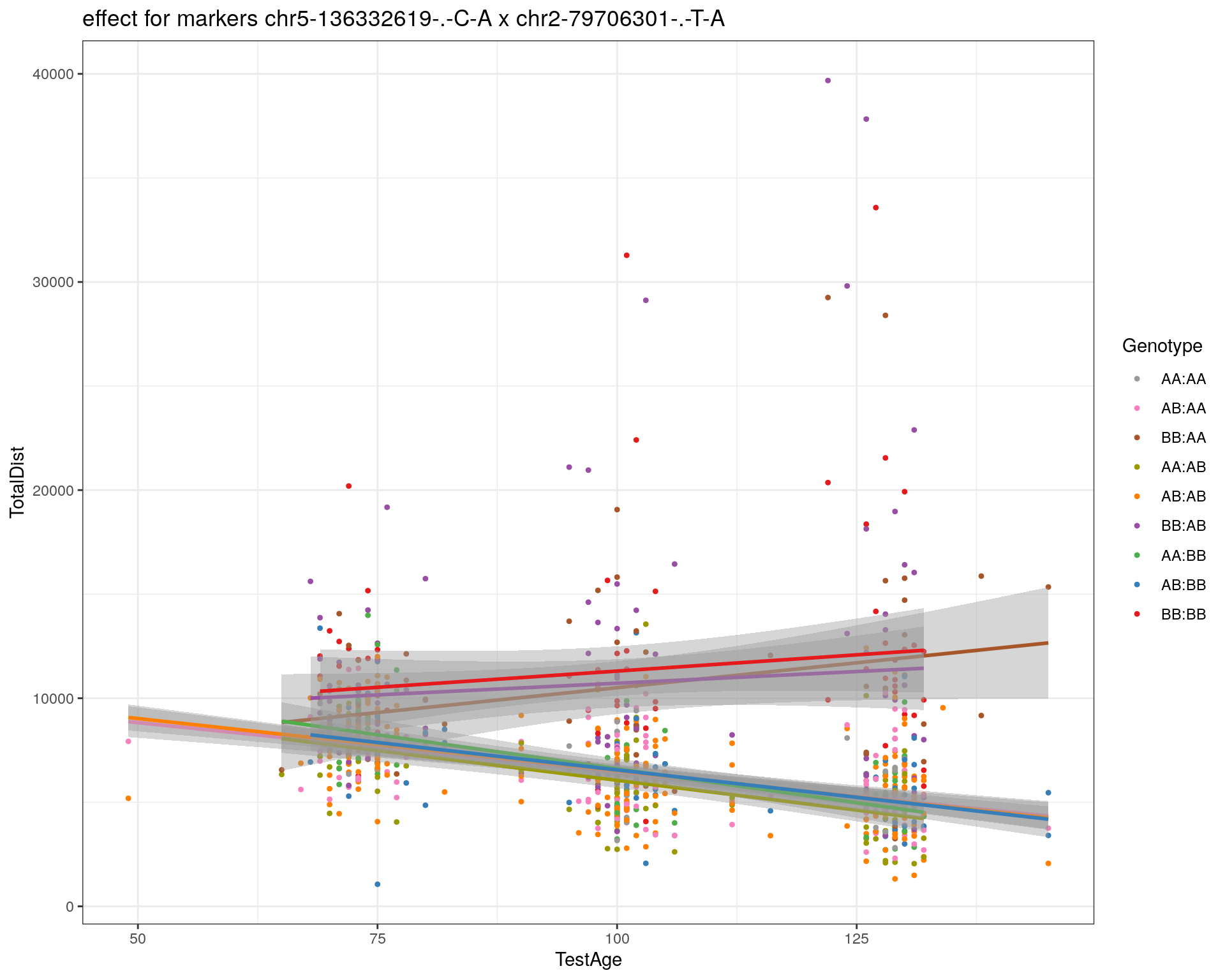
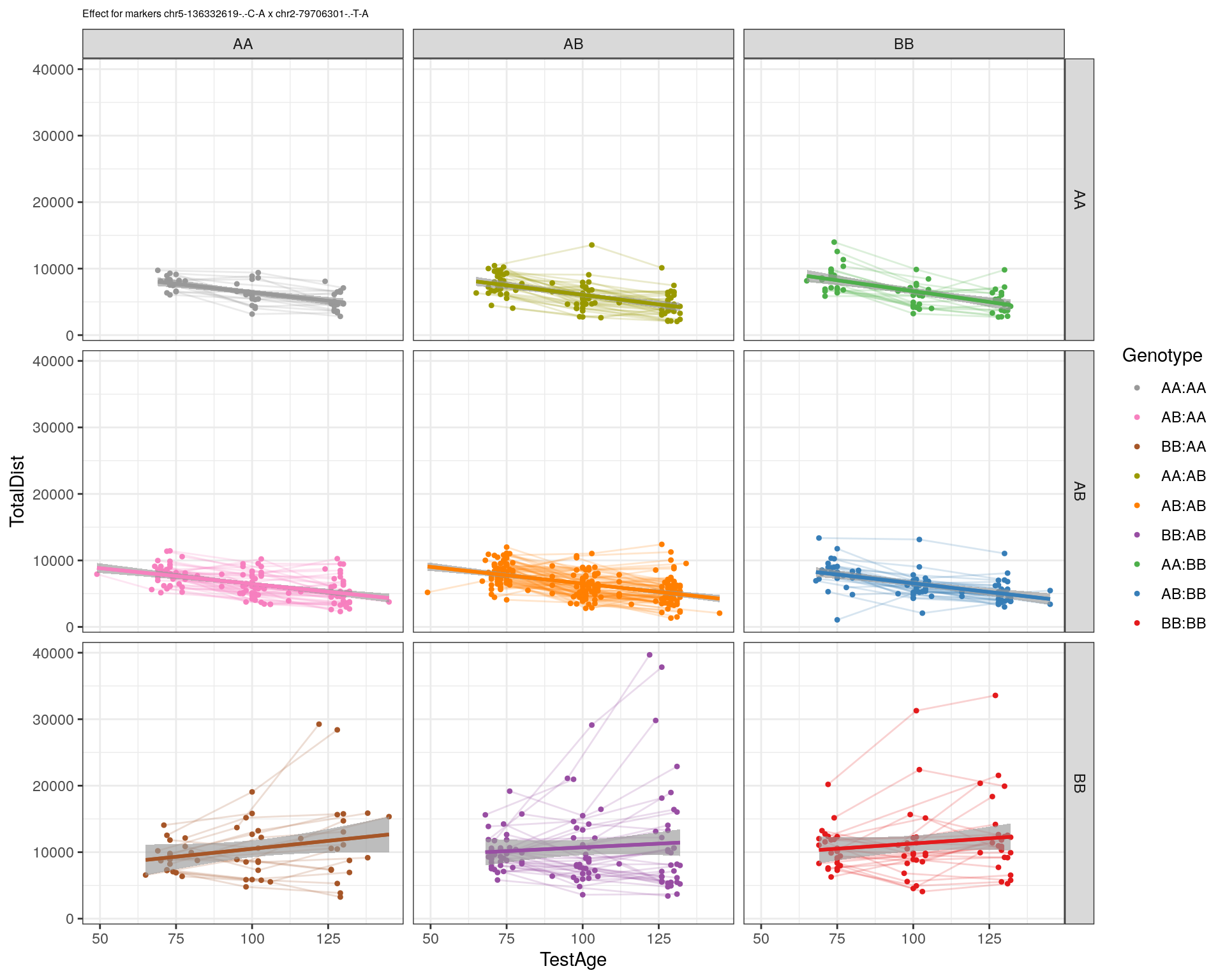
[1] "chr2-92367783-.-T-C"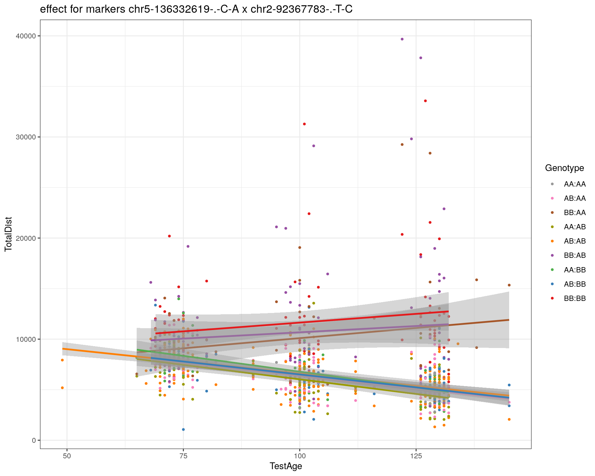
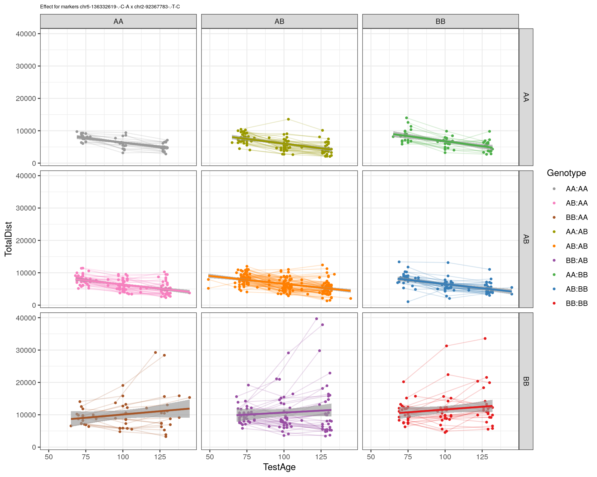
[1] "chr2-95118744-.-T-A"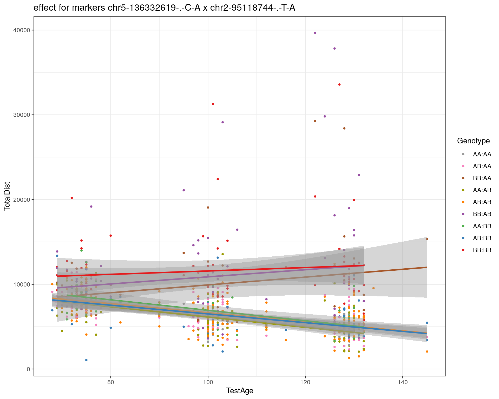
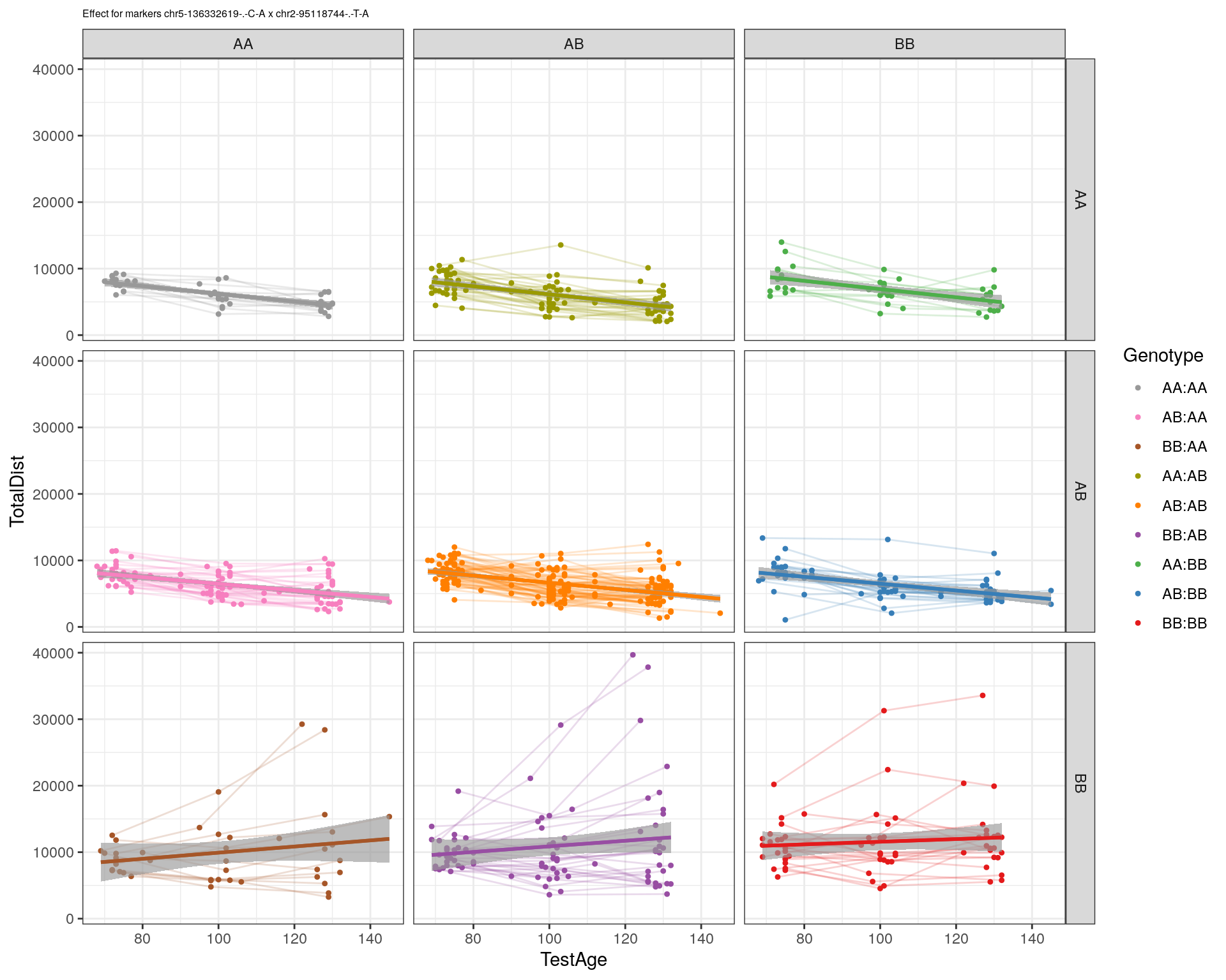
[1] "chr2-102169266-.-C-T"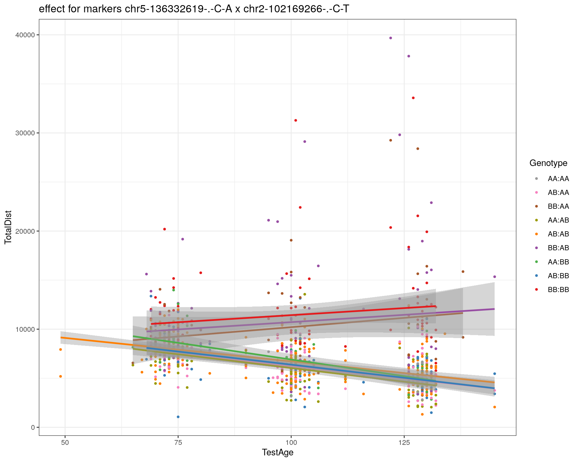
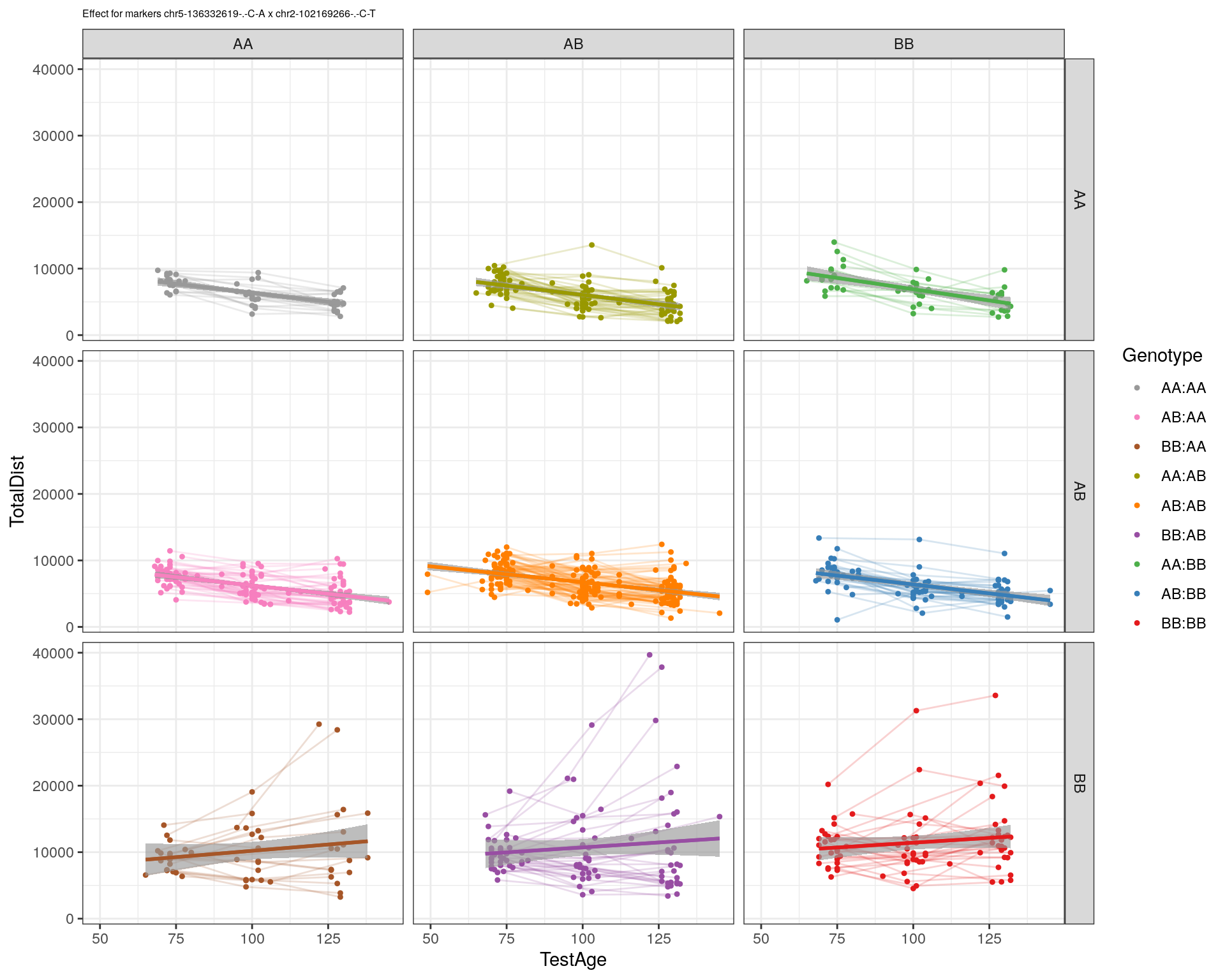
[1] "chr2-130405980-.-A-T"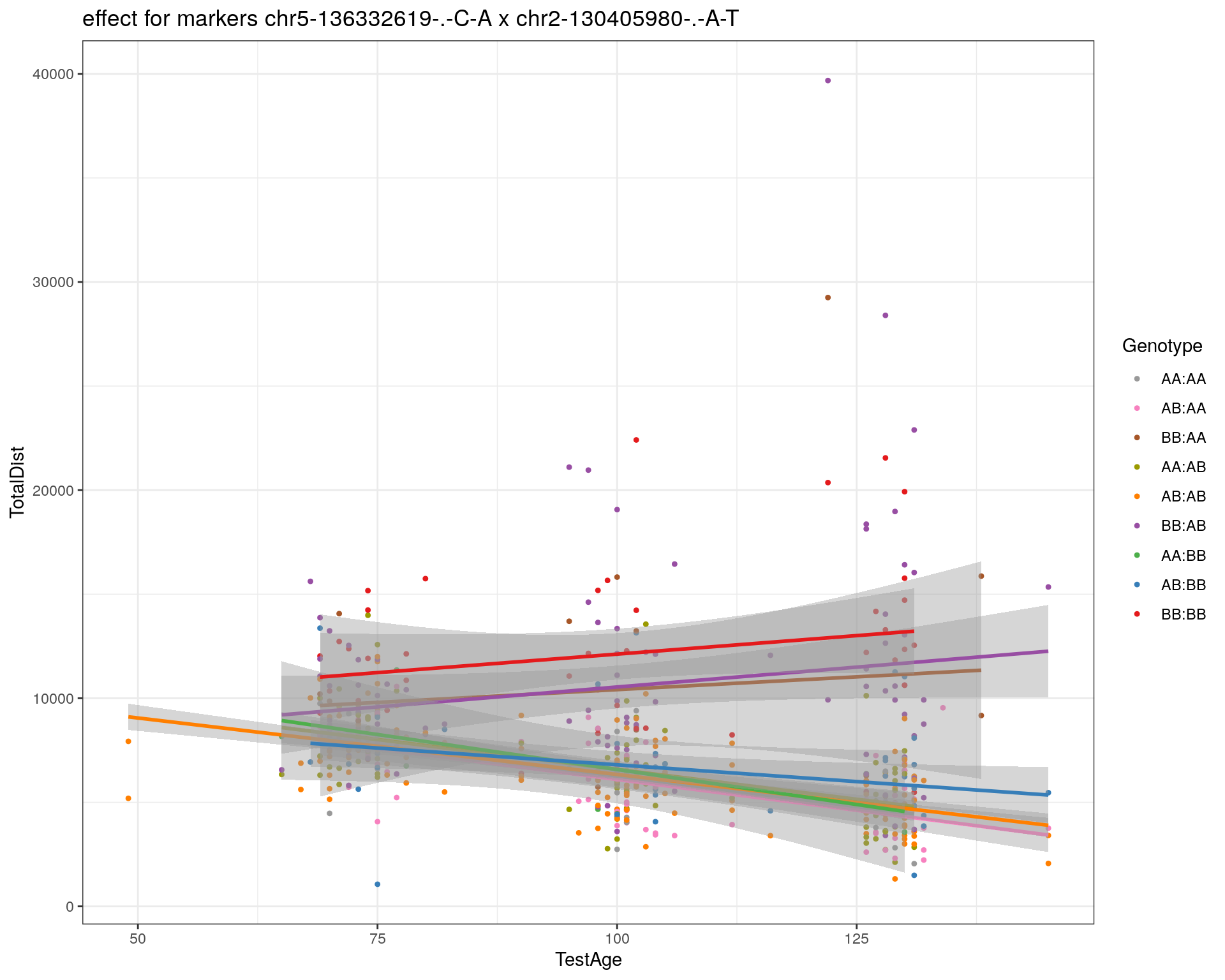
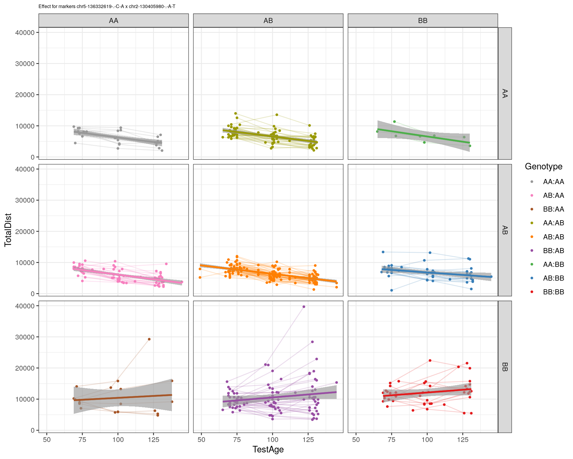
[1] "chr2-137498061-.-T-A"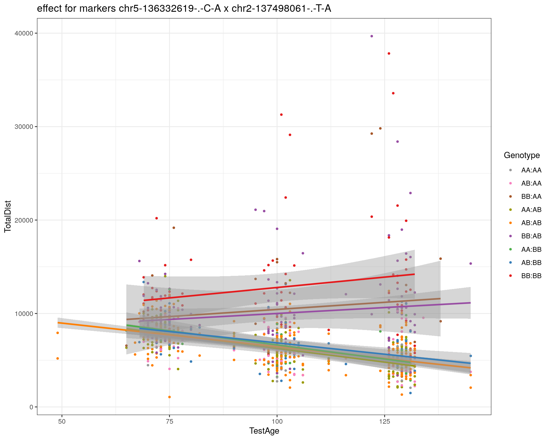
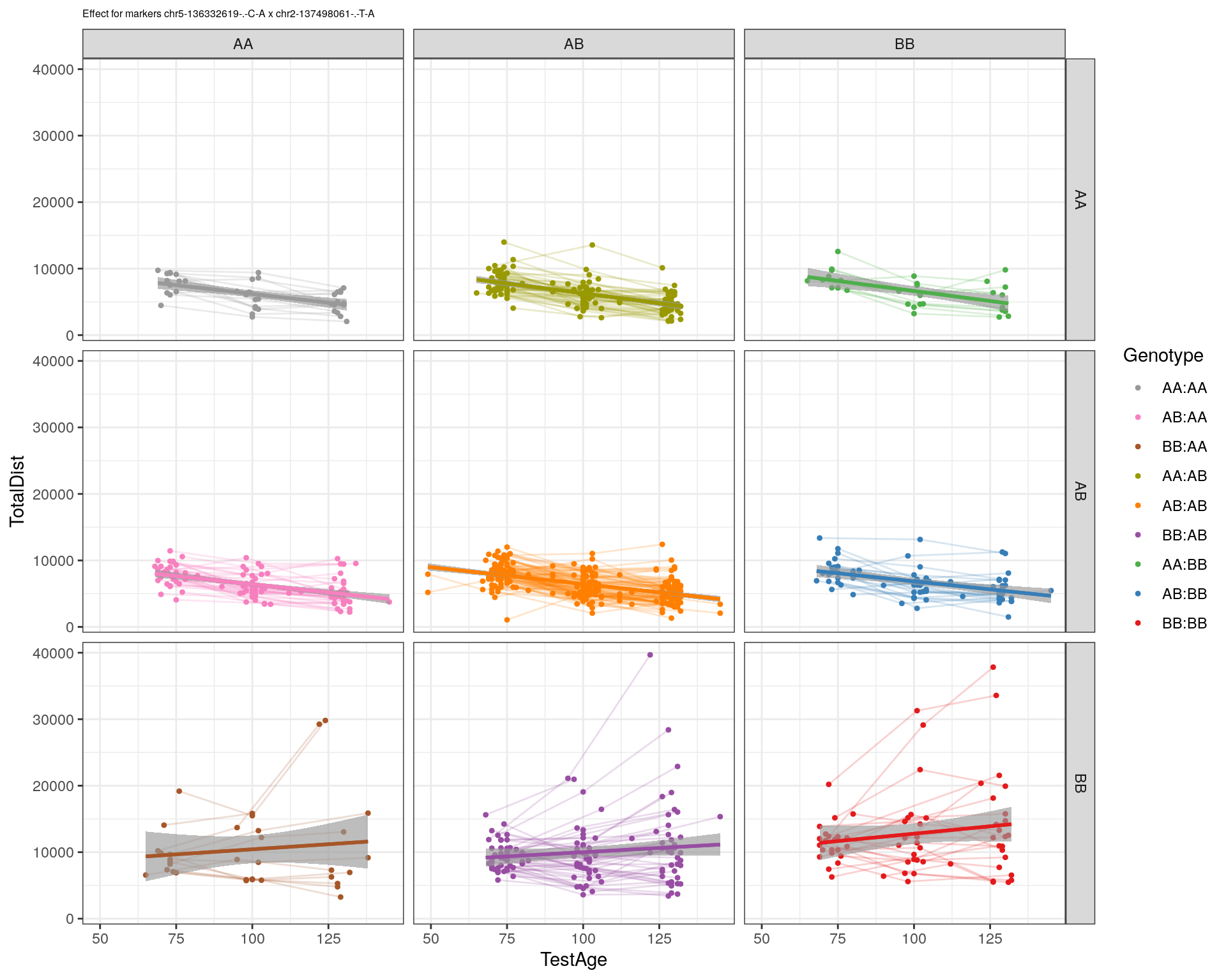
[1] "chr2-145128463-.-A-T"
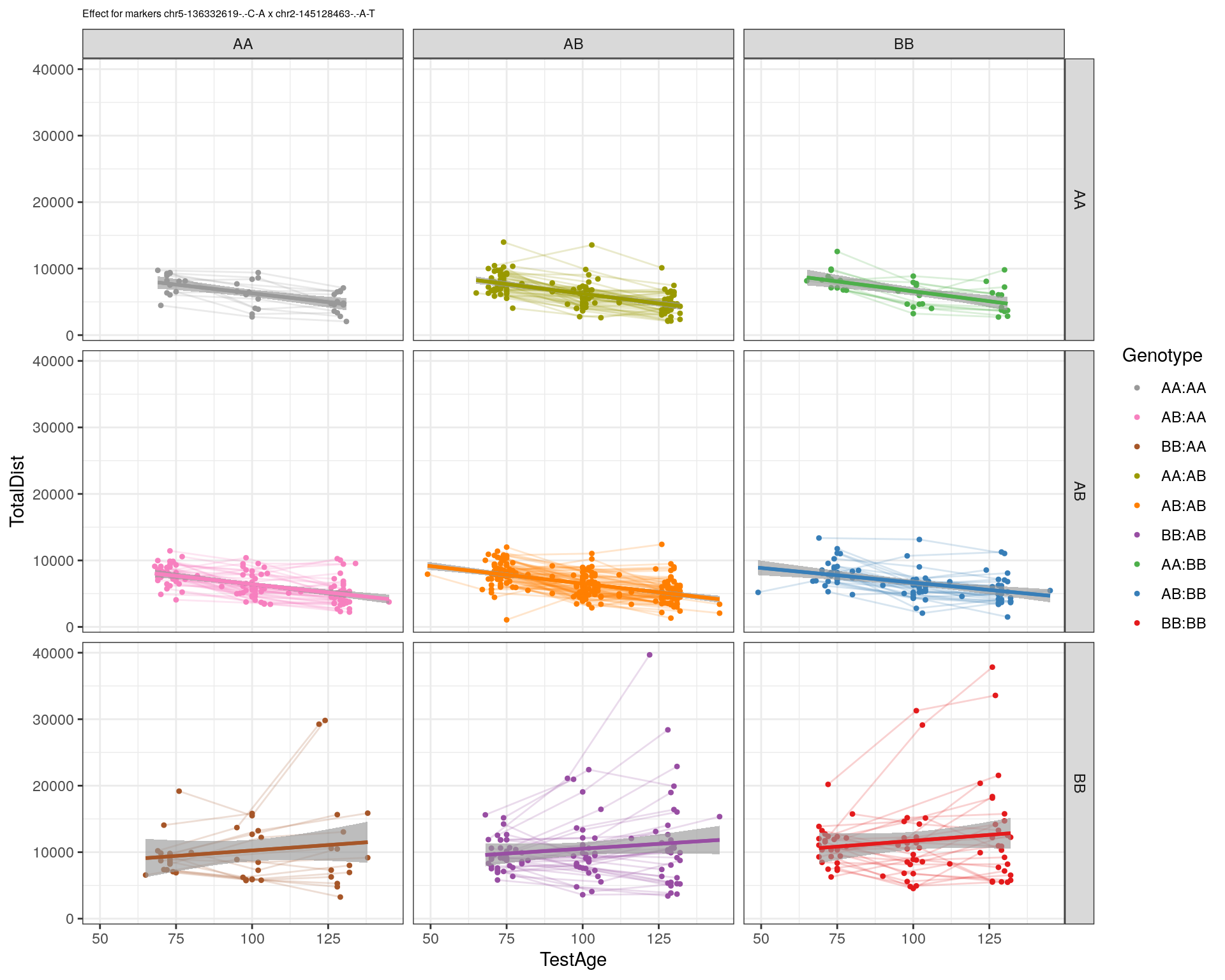
[1] "chr3-59218564-.-T-A"
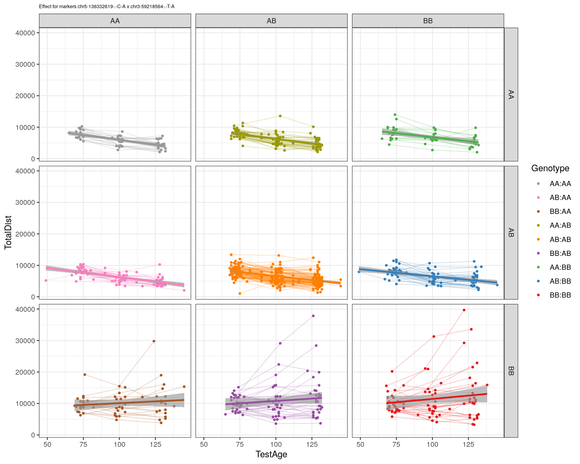
[1] "chr3-98881230-.-G-A"
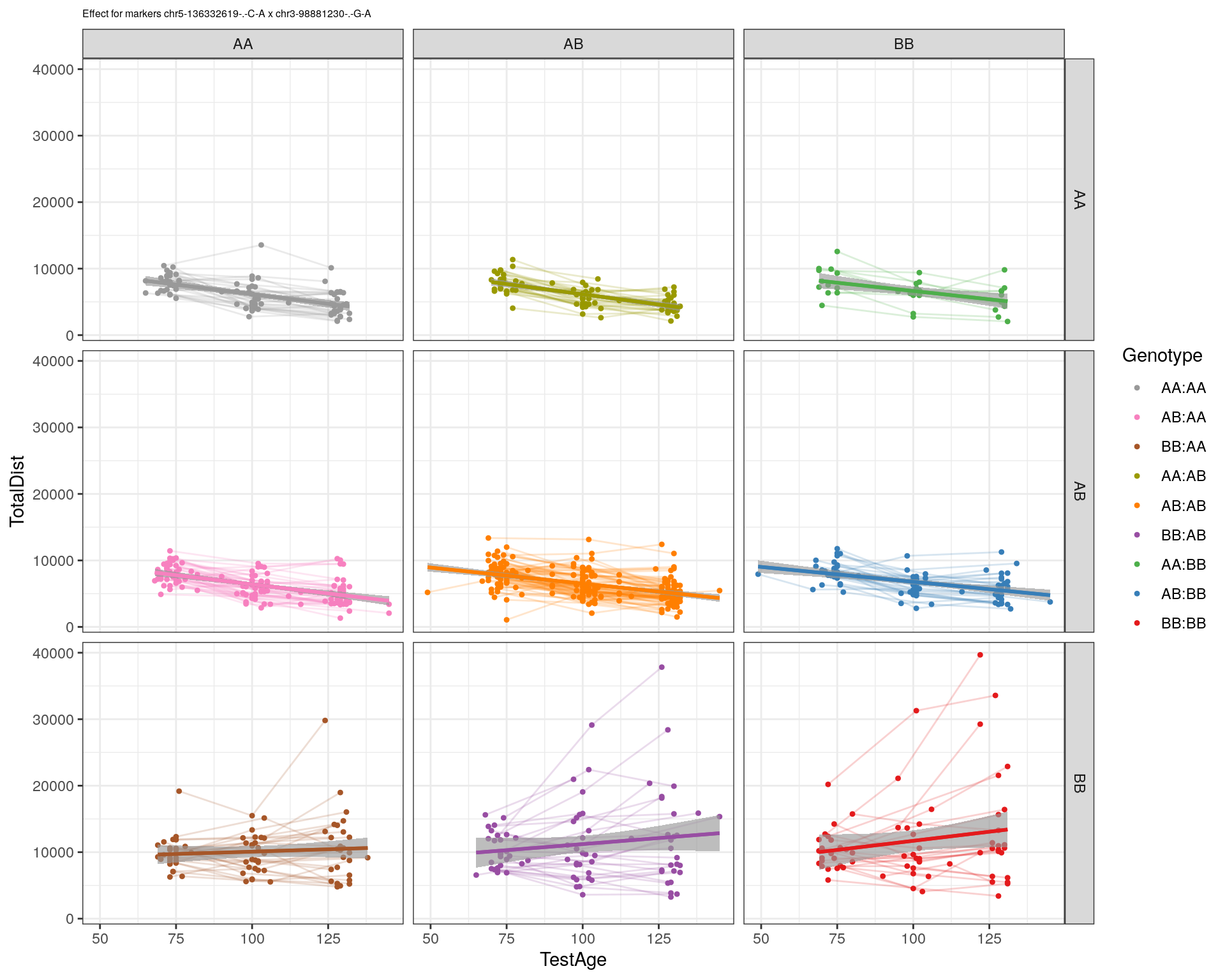
[1] "chr3-106985708-.-A-C"
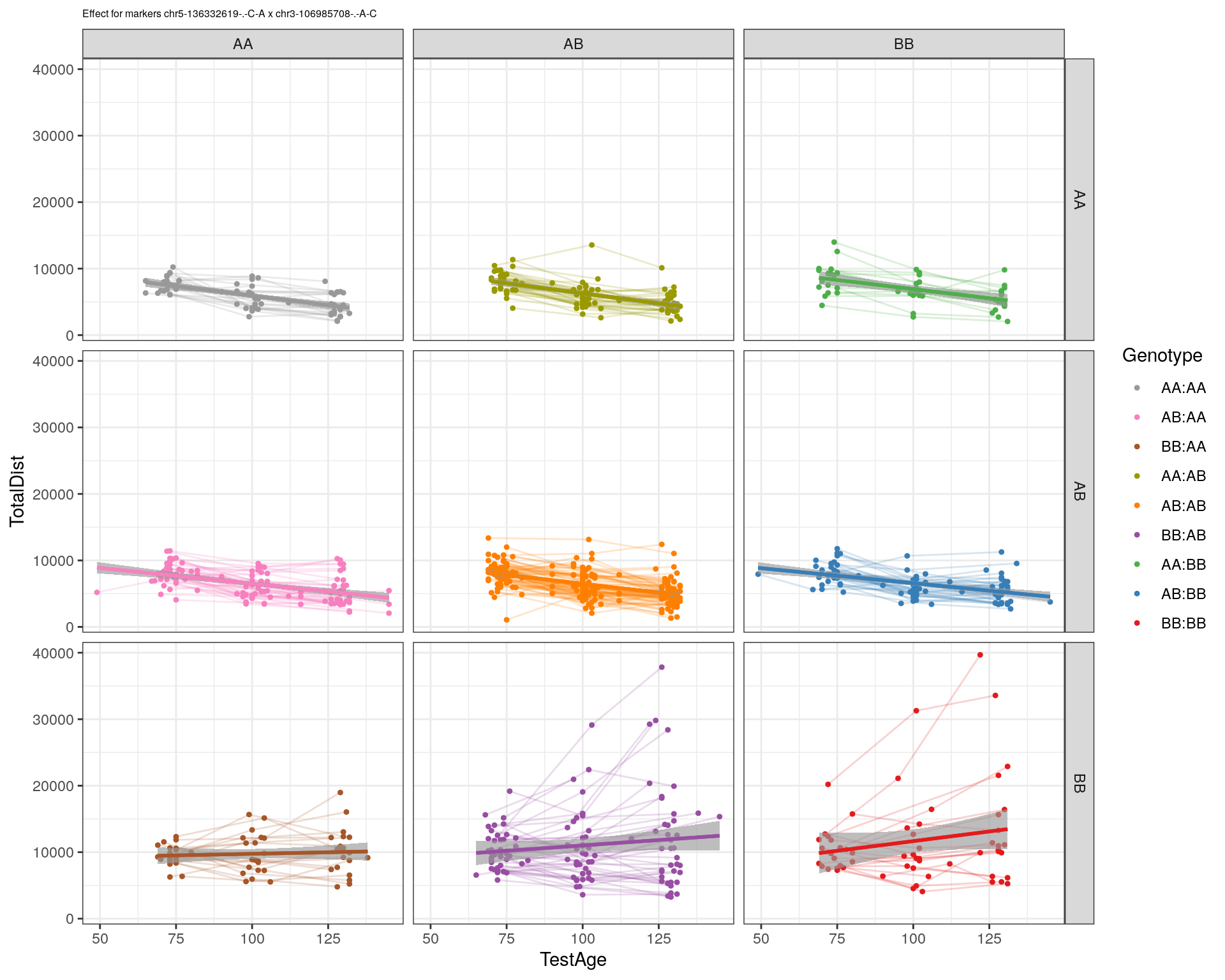
[1] "chr3-135614002-.-T-G"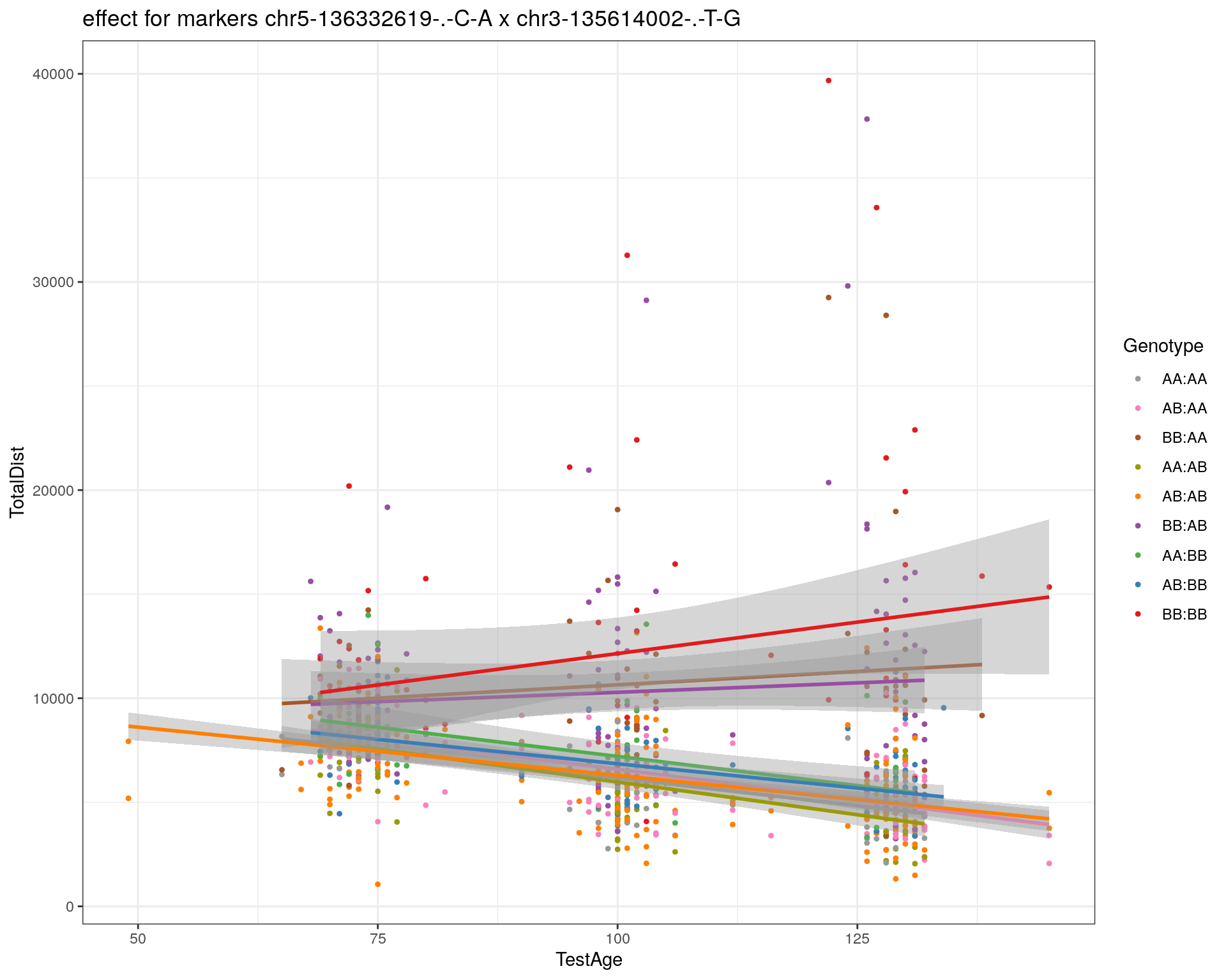

[1] "chr3-145286160-.-C-A"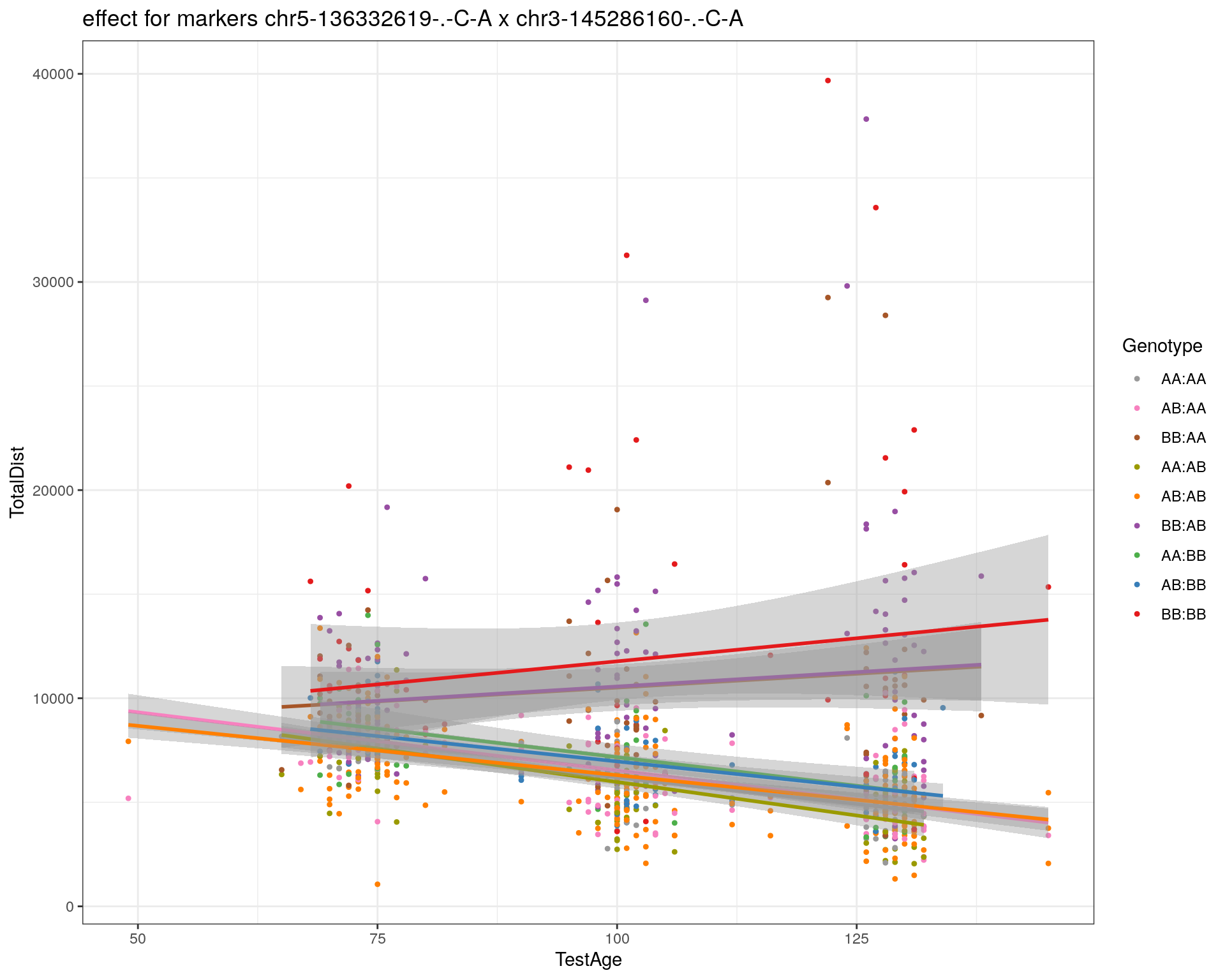

[1] "chr3-146750531-.-A-G"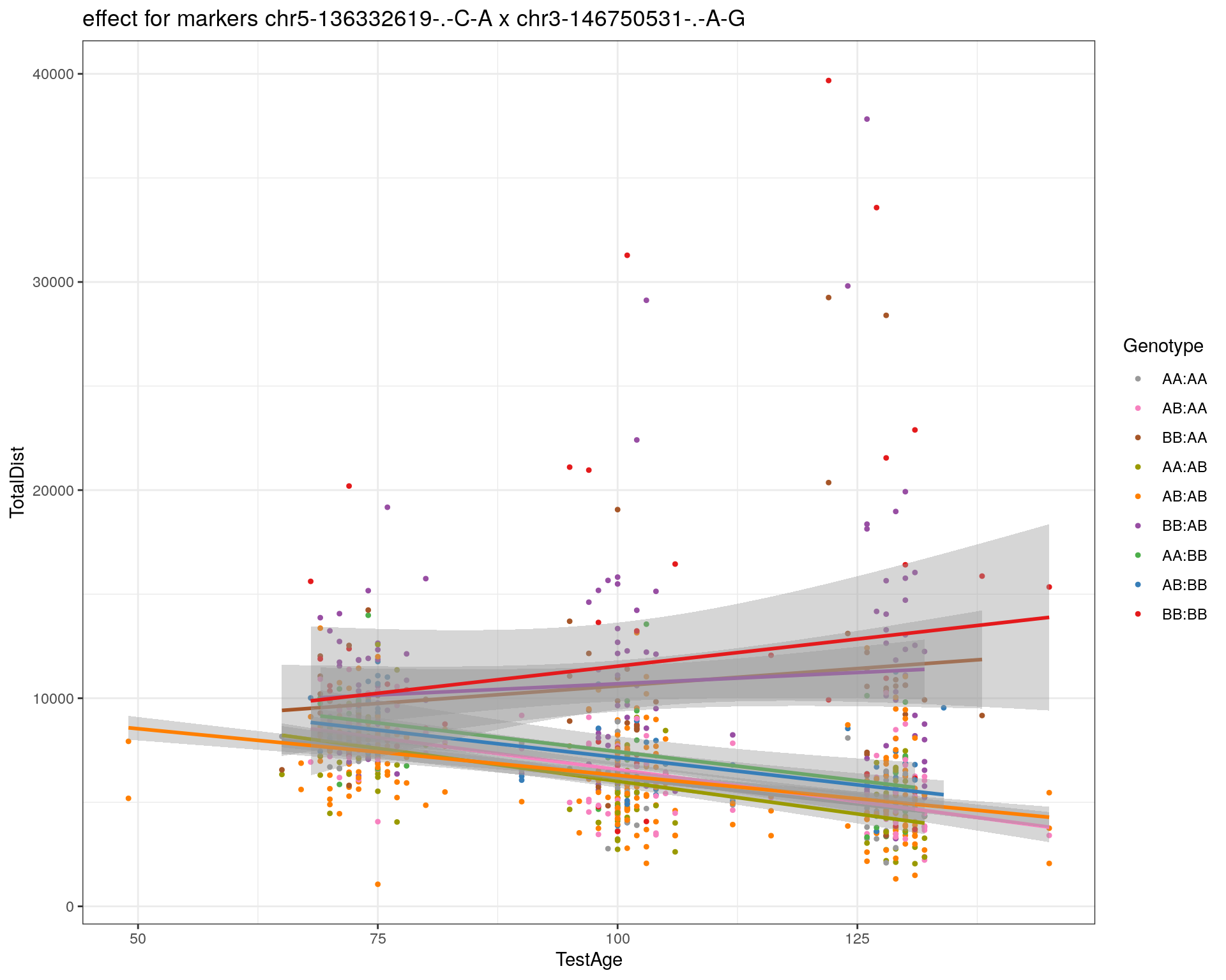
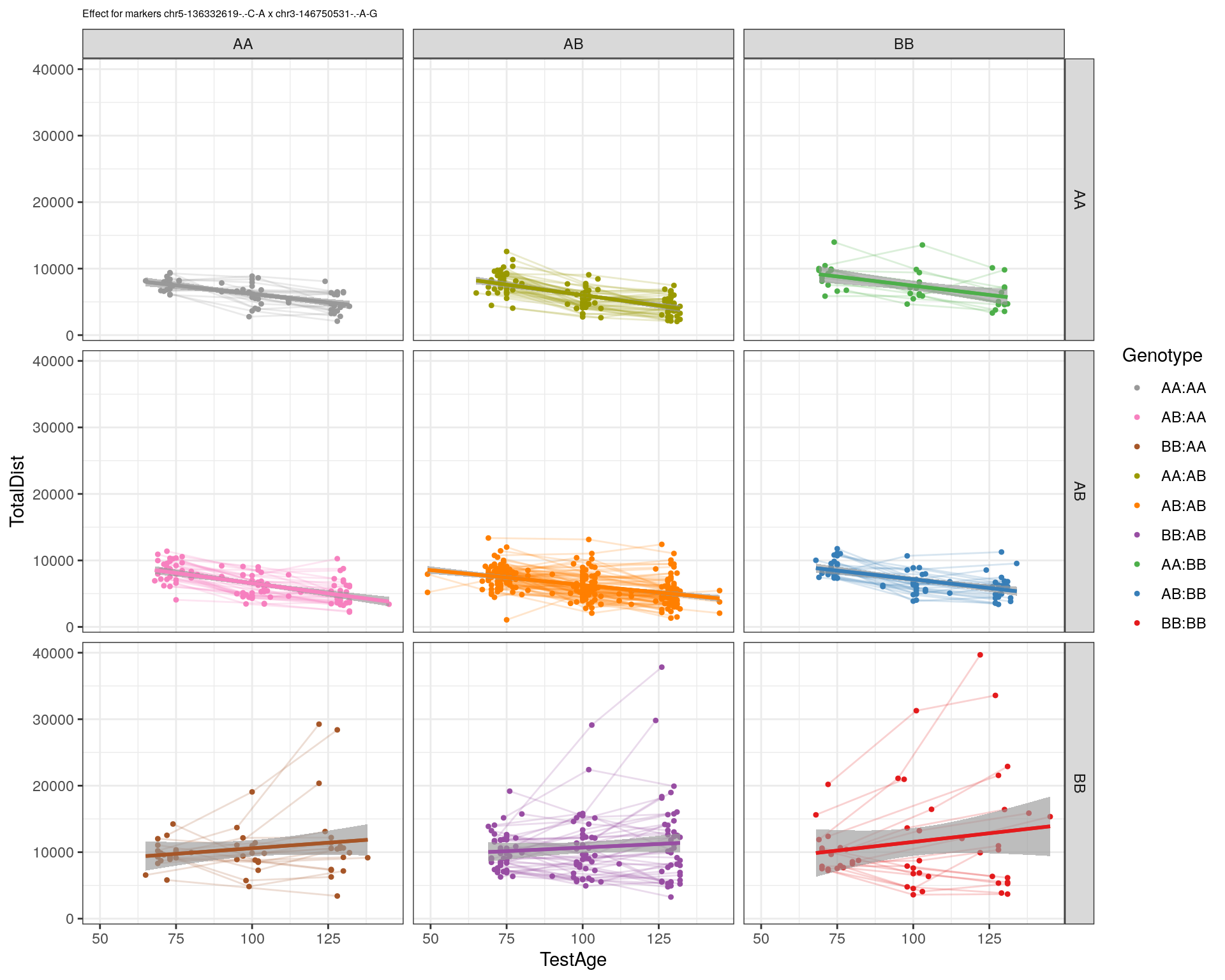
[1] "chr3-152699551-.-G-A"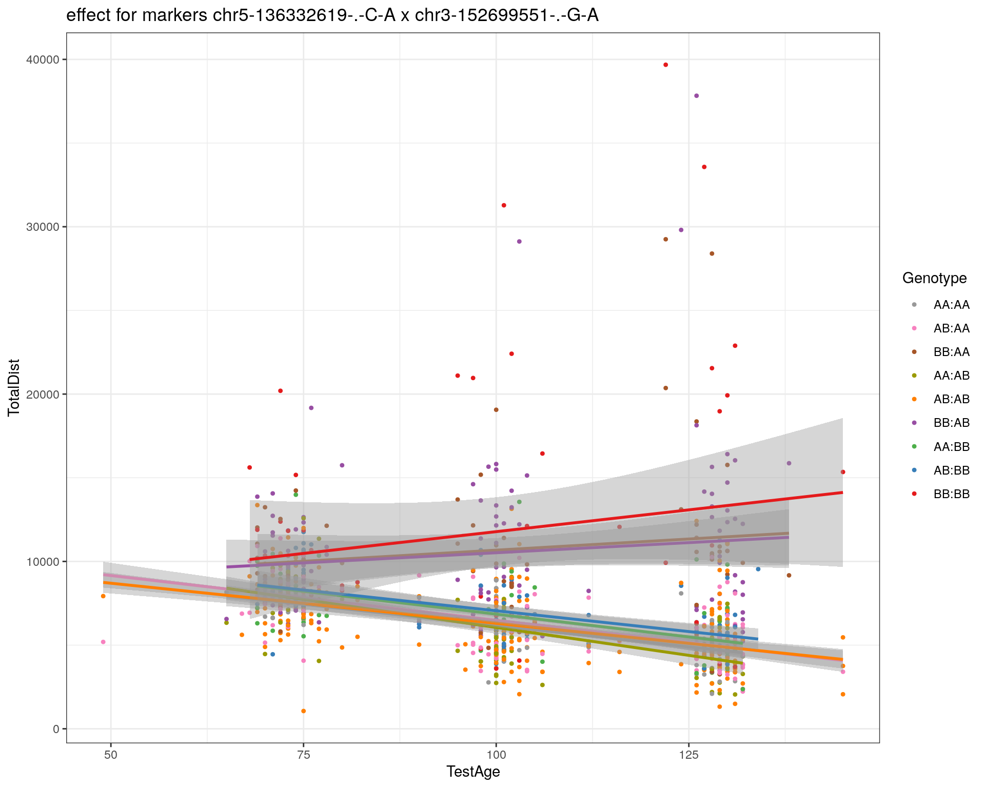
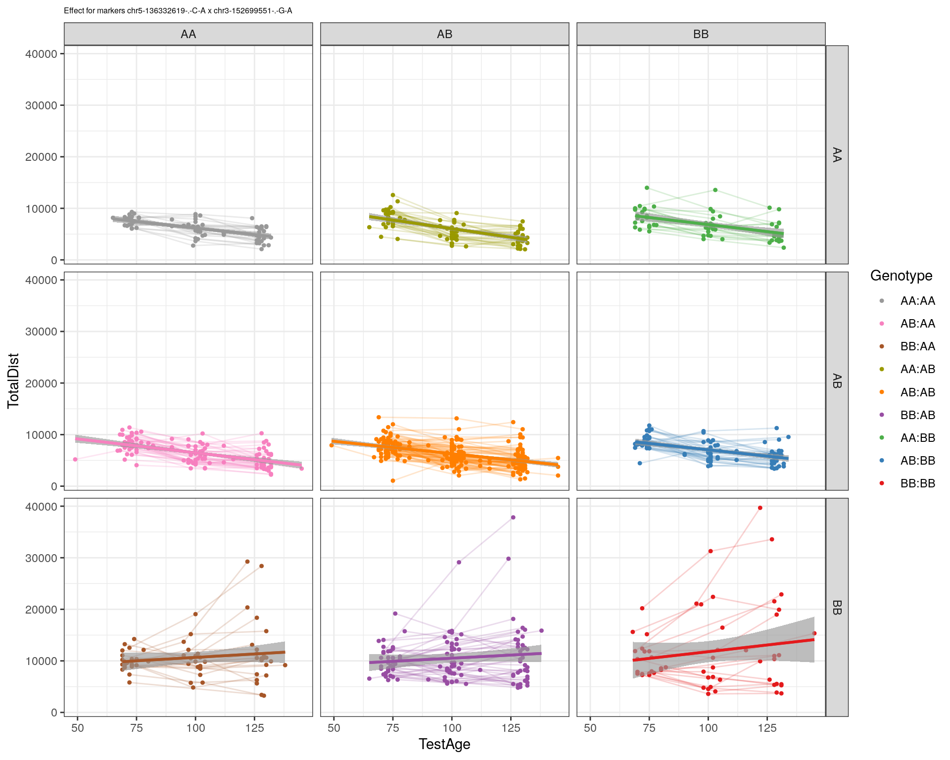
[1] "chr4-32821418-.-C-T"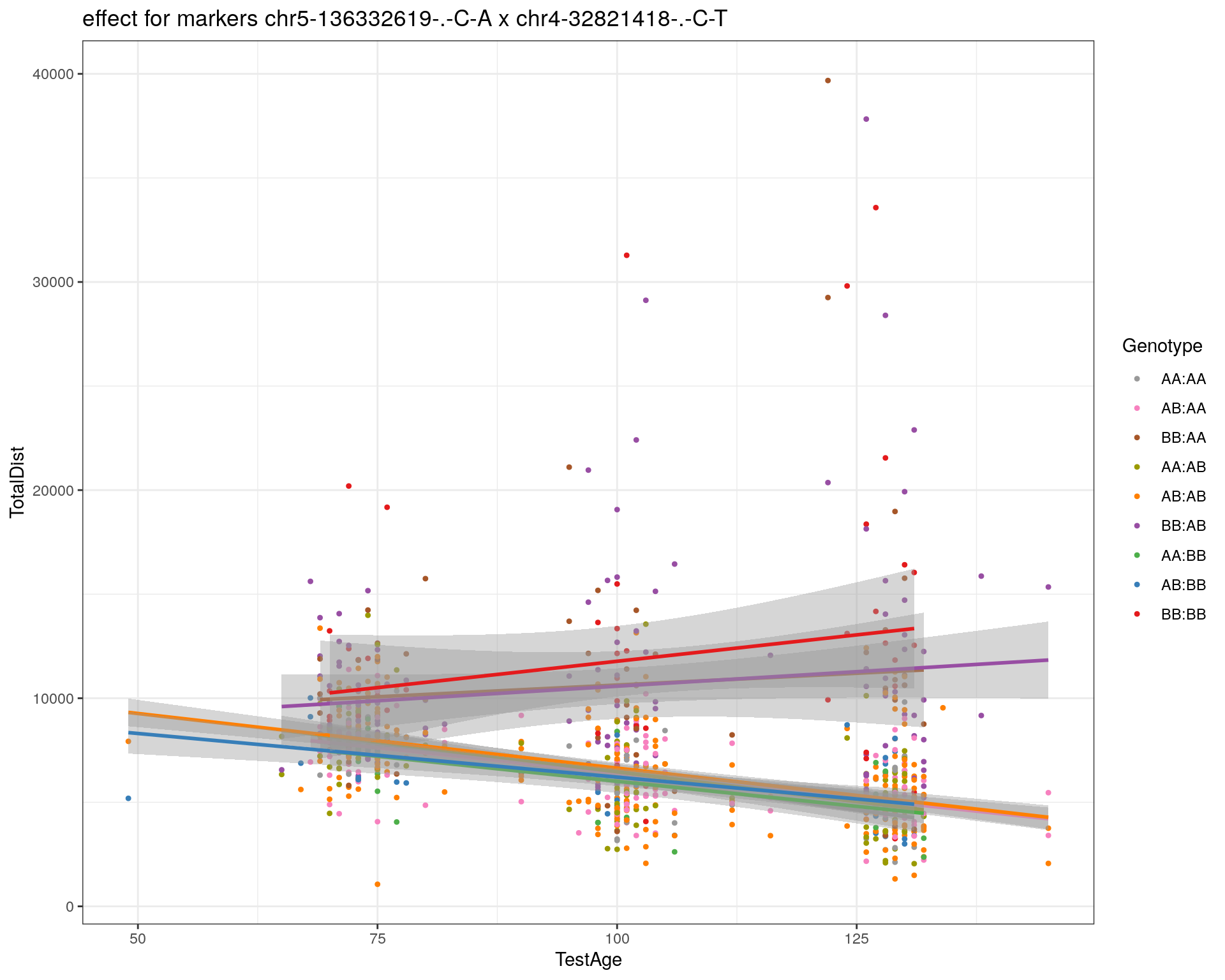
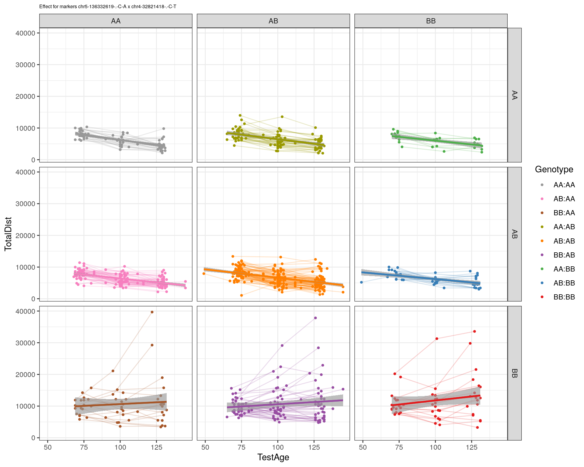
[1] "chr5-75264187-.-T-C"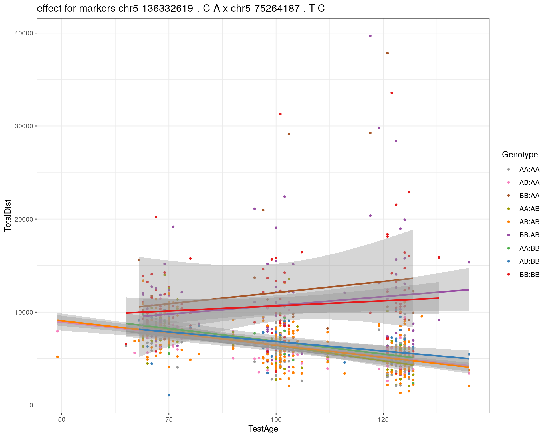
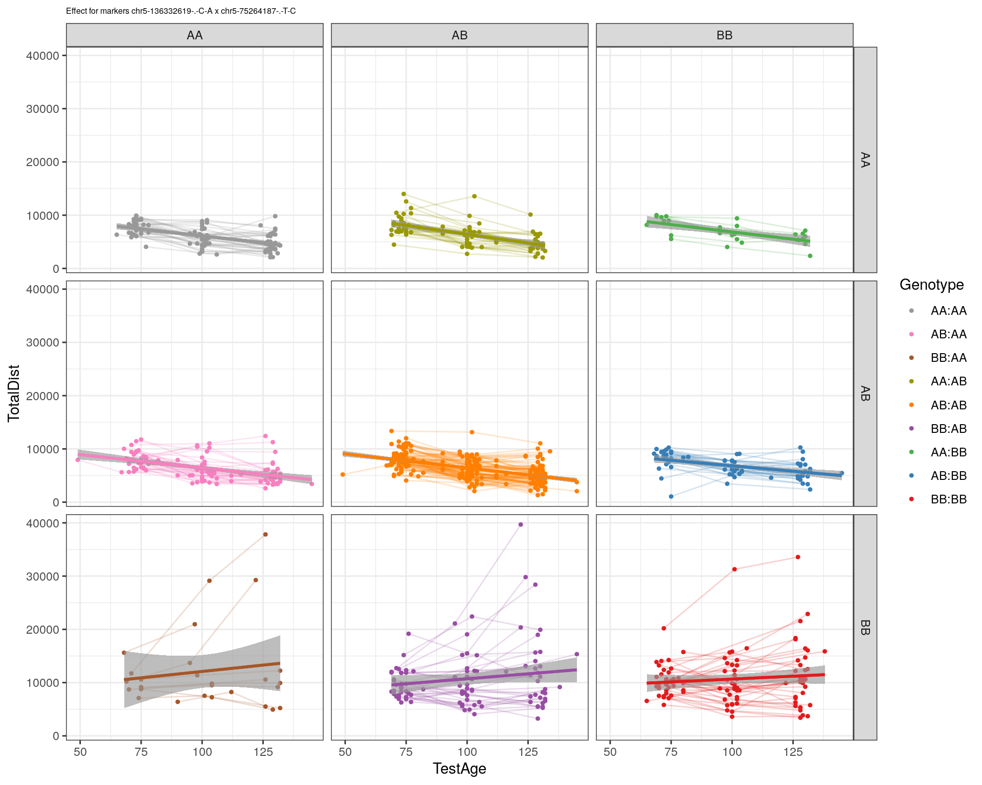
[1] "chr5-90233933-.-A-T"
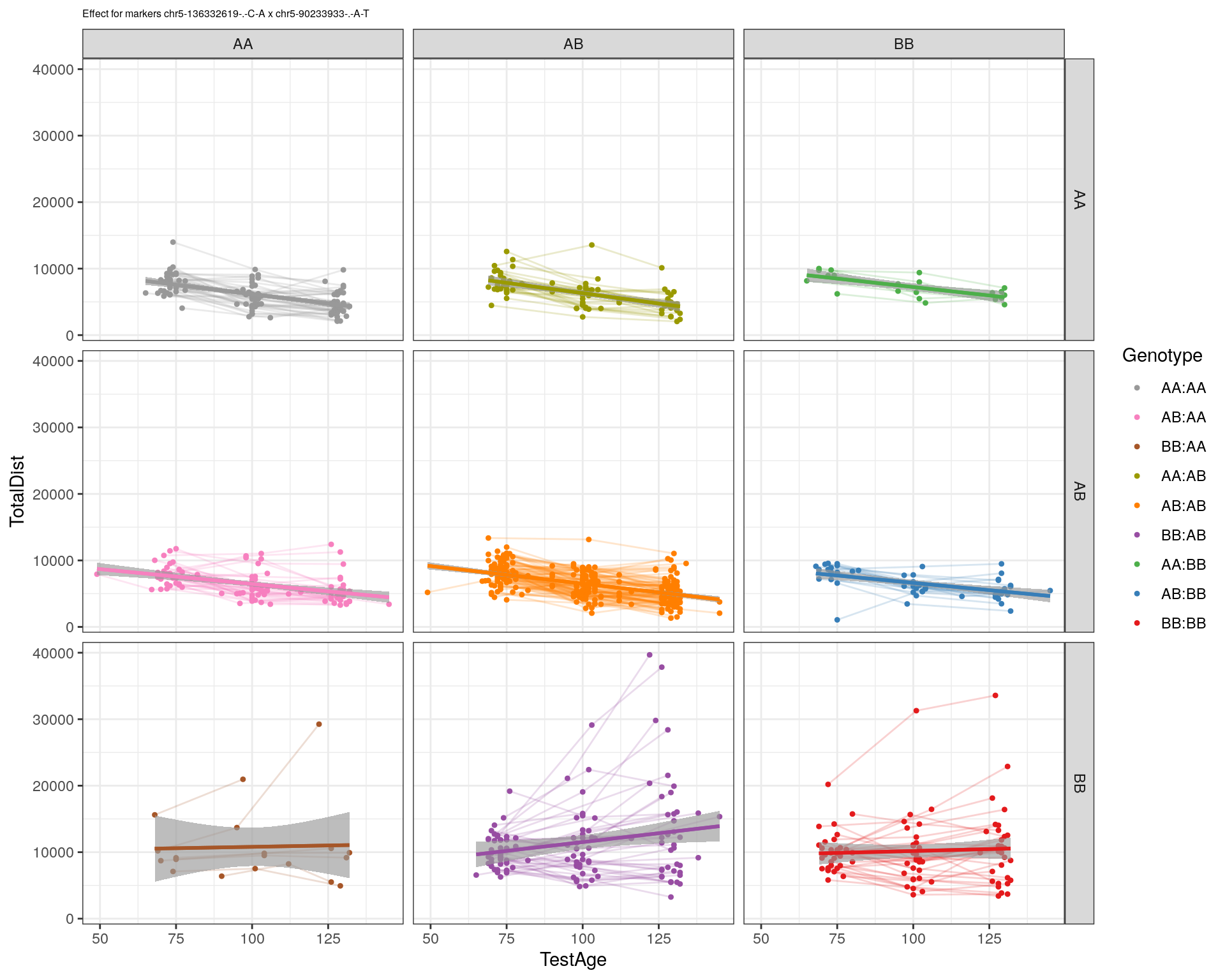
[1] "chr5-97607237-.-T-A"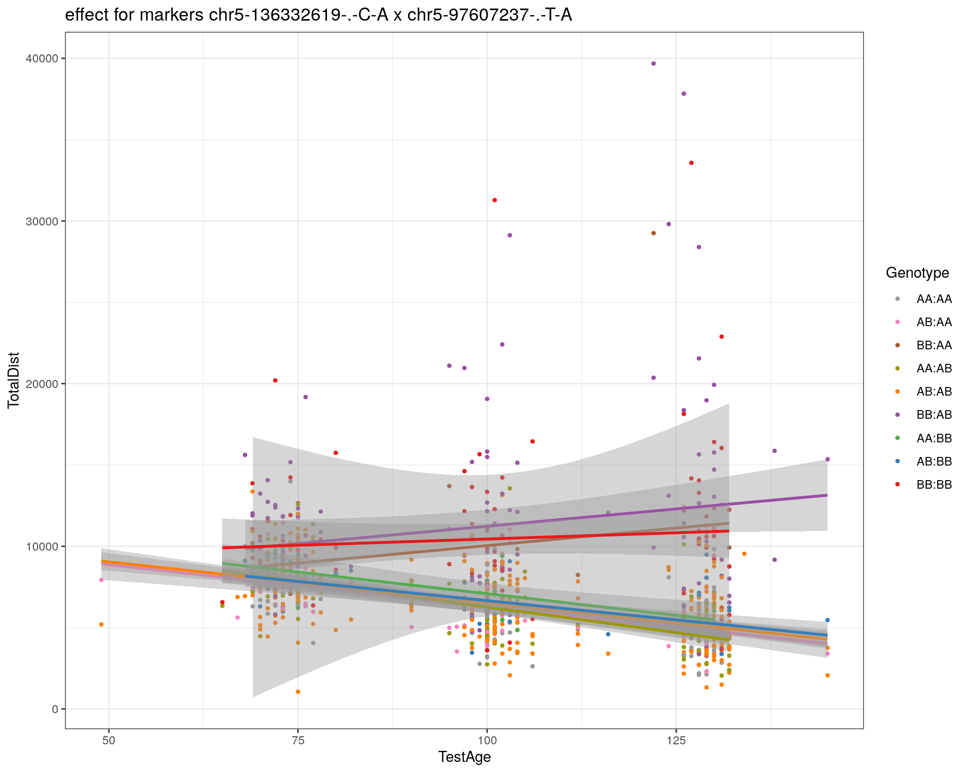
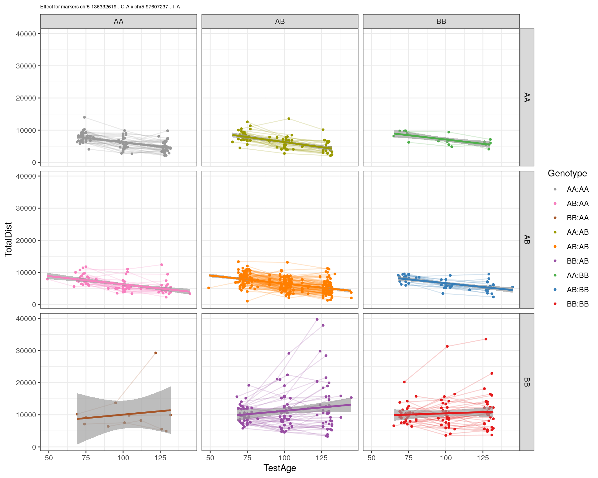
[1] "chr5-107507008-.-C-T"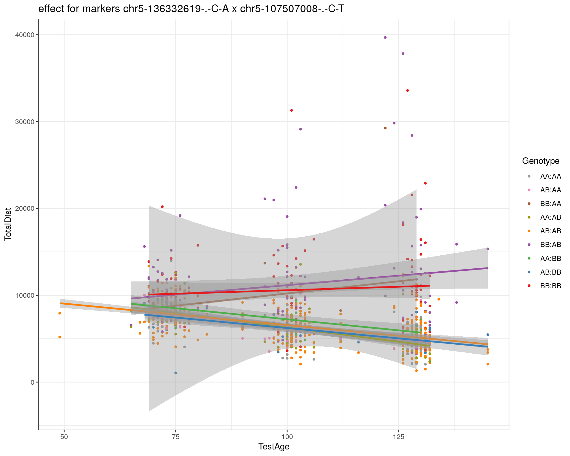
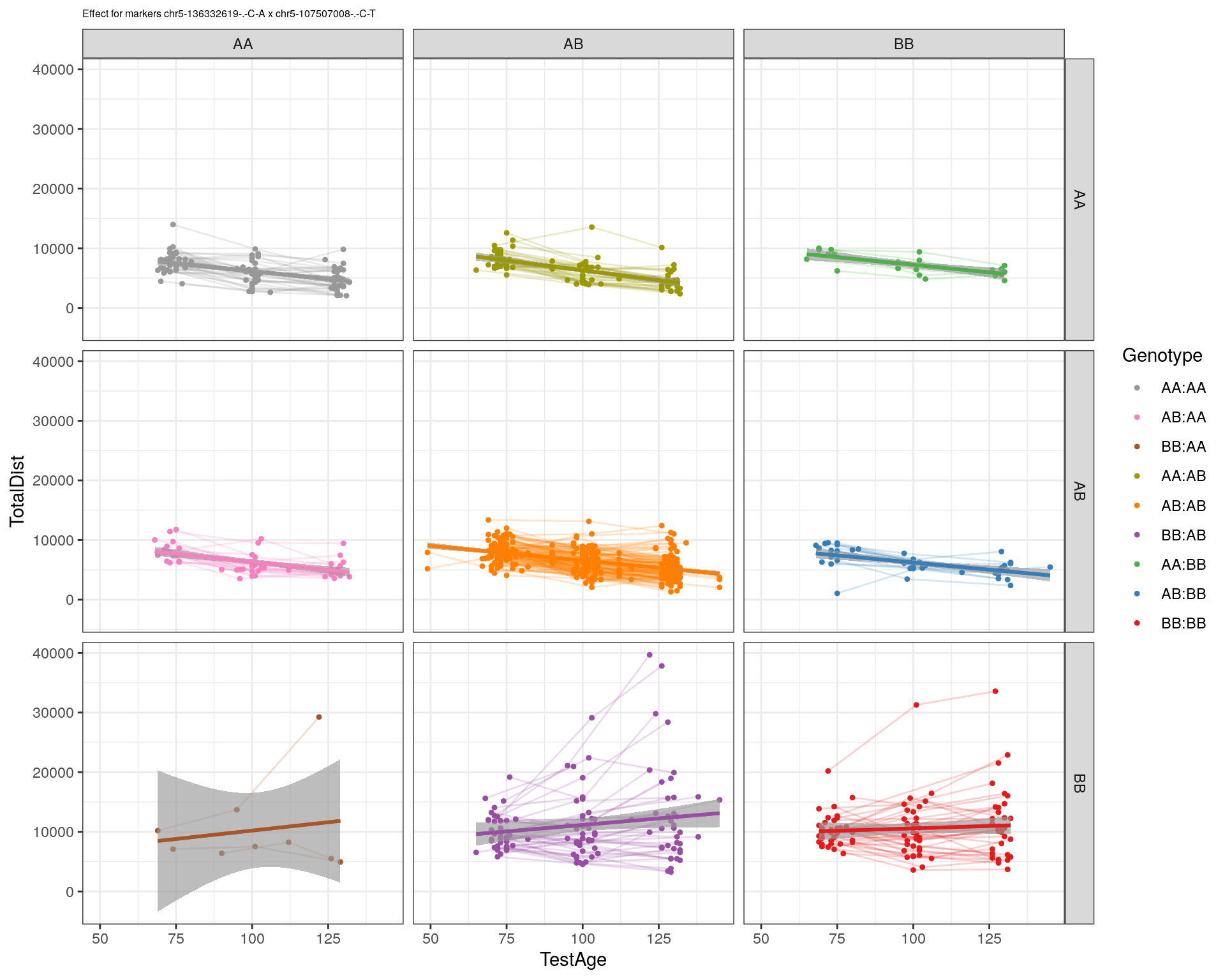
[1] "chr5-112799362-.-C-T"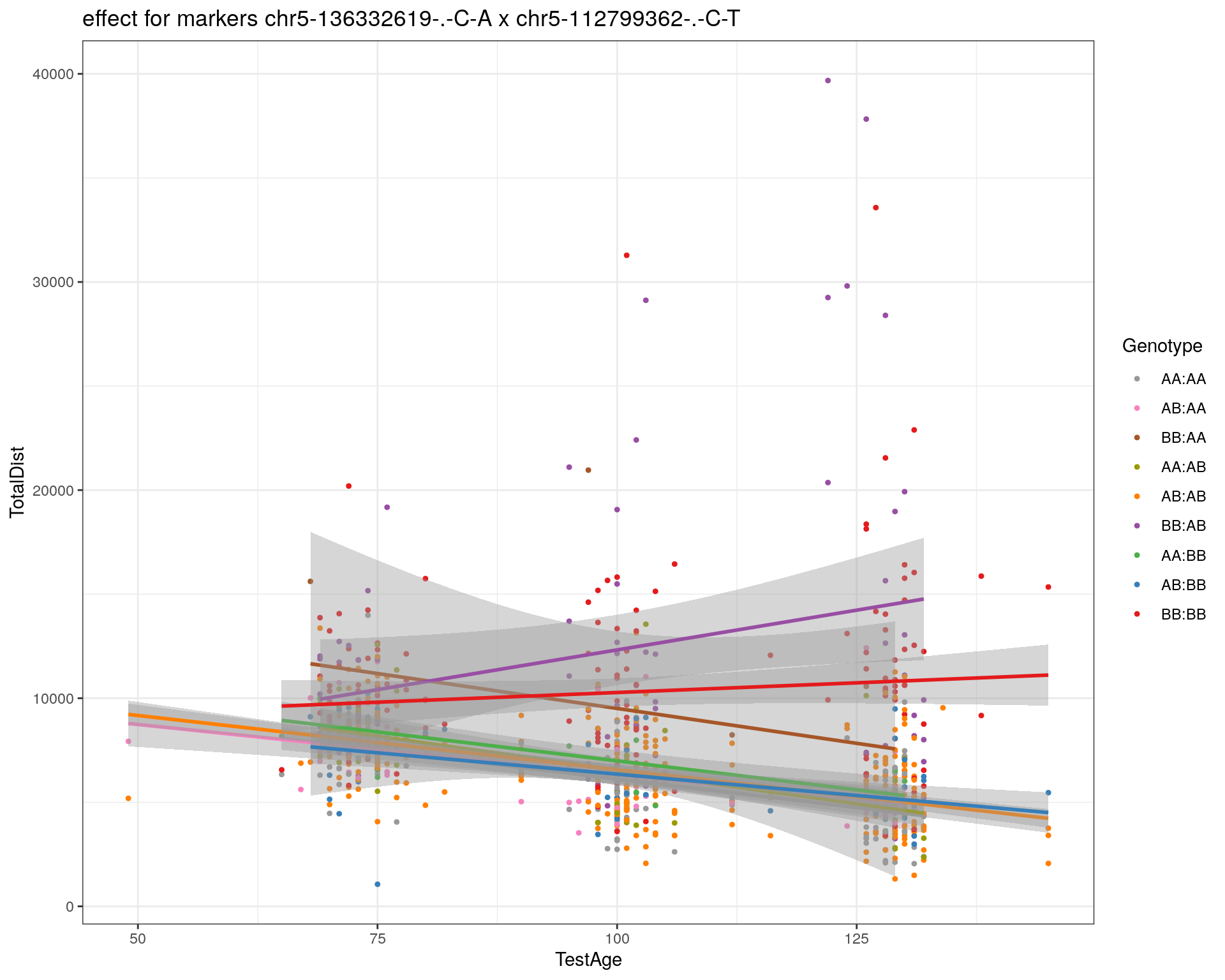
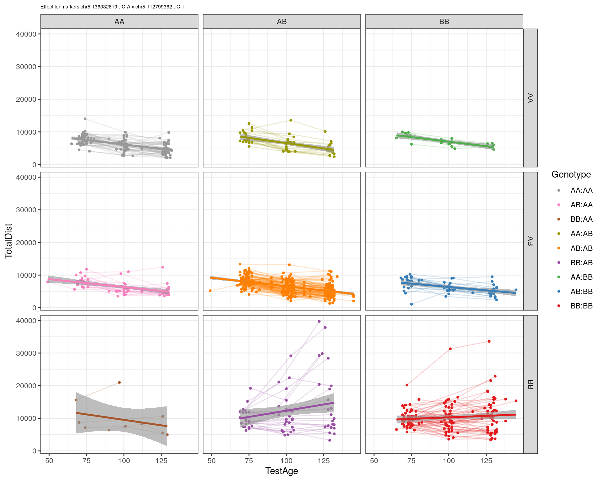
[1] "chr5-120660771-.-T-A"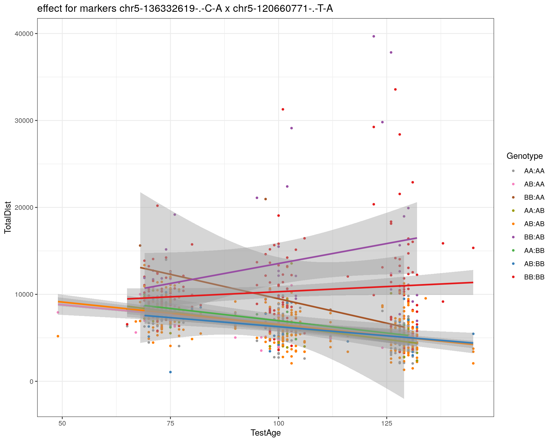
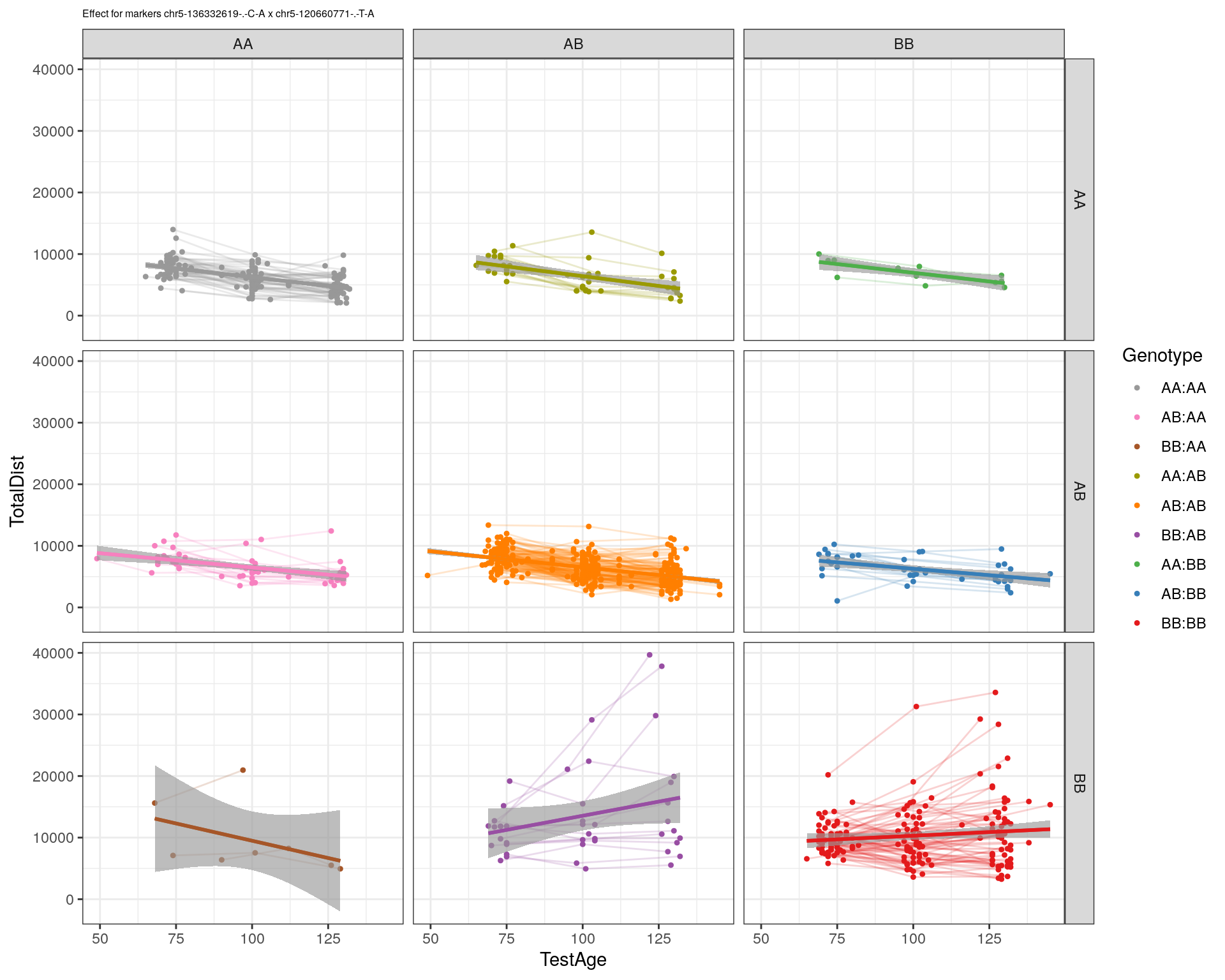
[1] "chr5-122167749-.-T-C"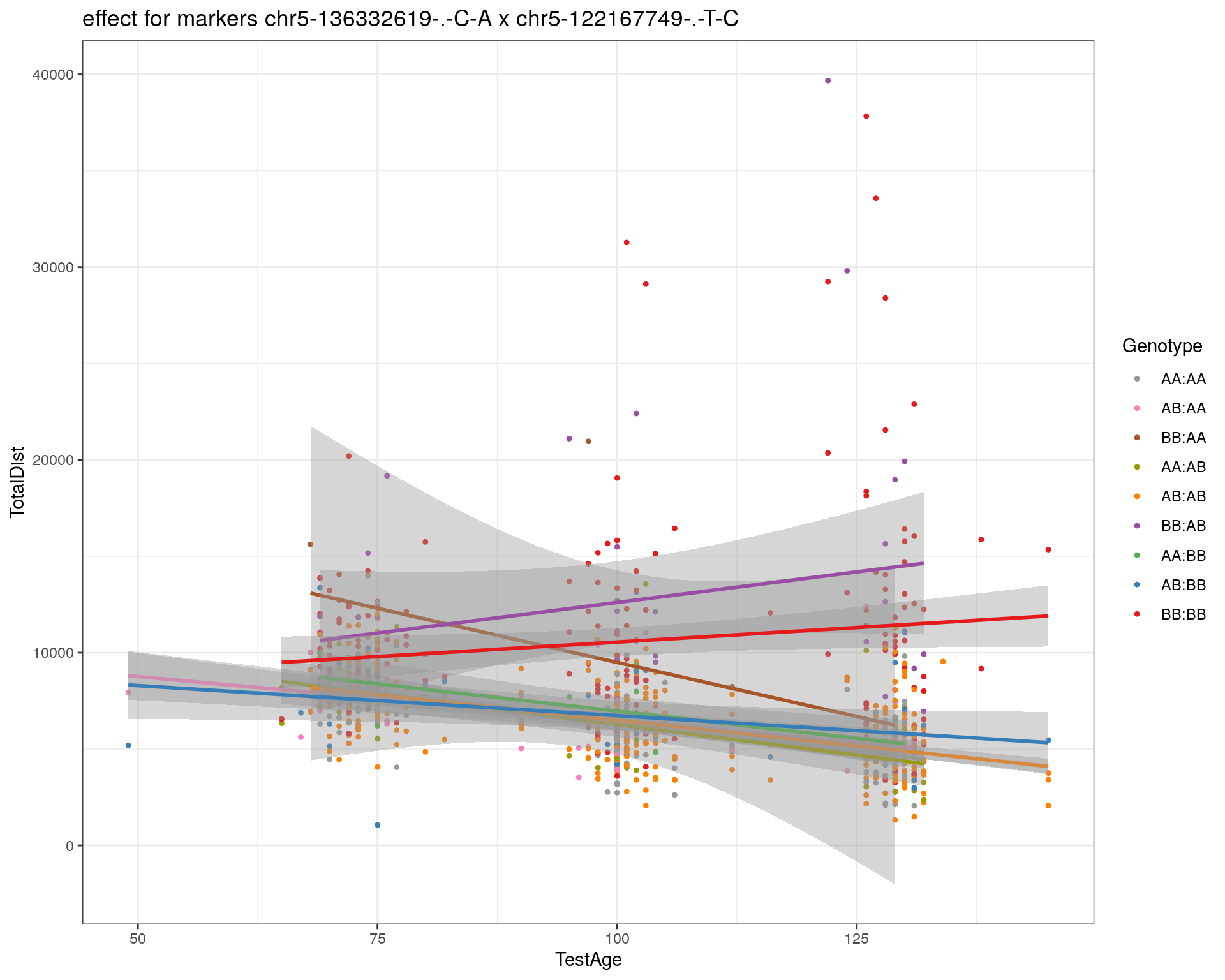

[1] "chr5-125153901-.-C-T"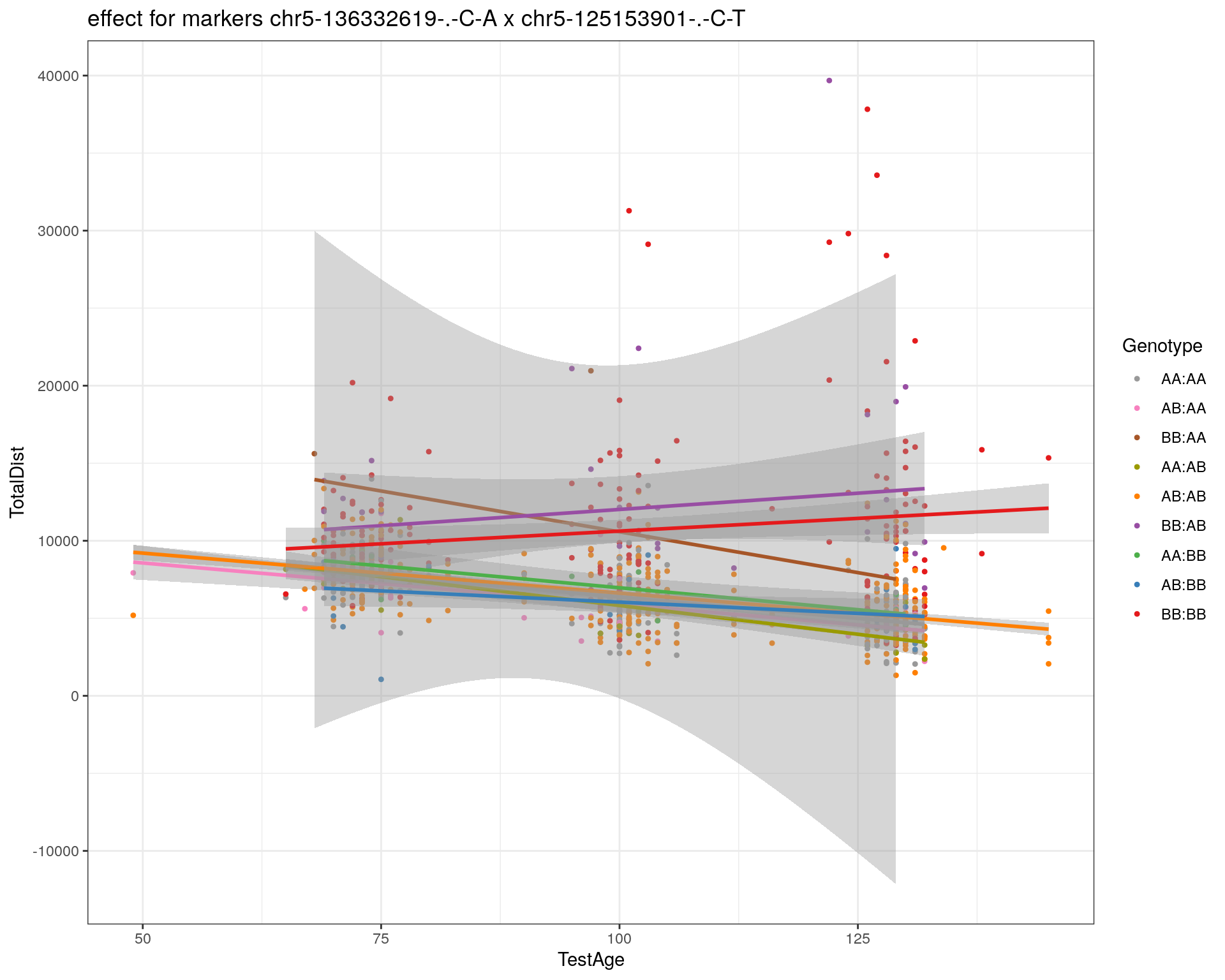
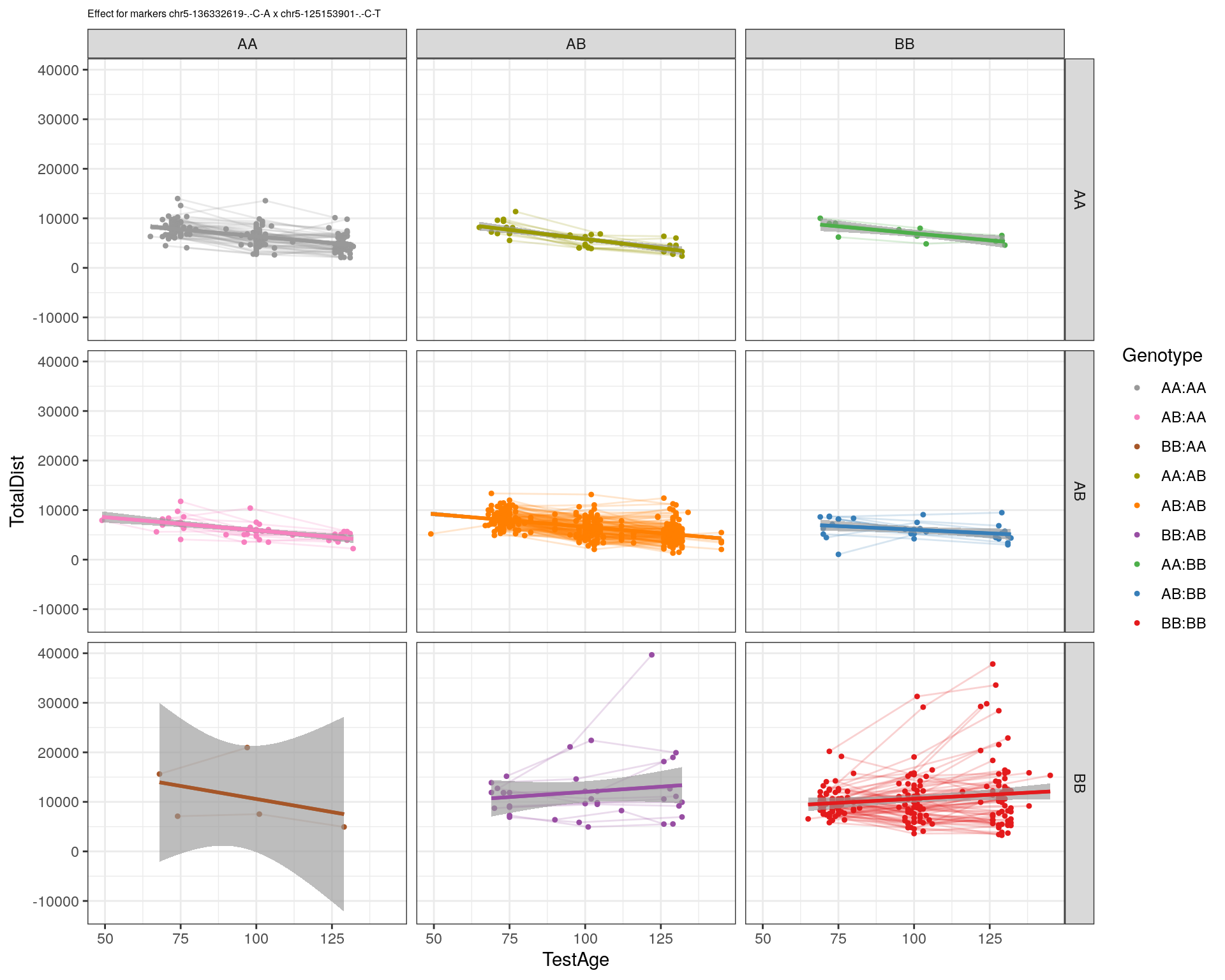
[1] "chr5-126058493-.-T-A"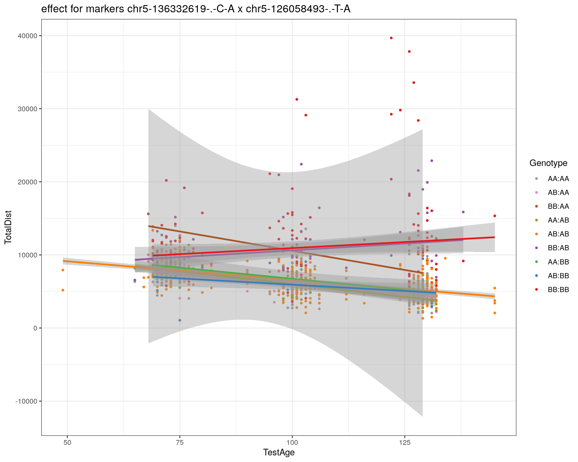
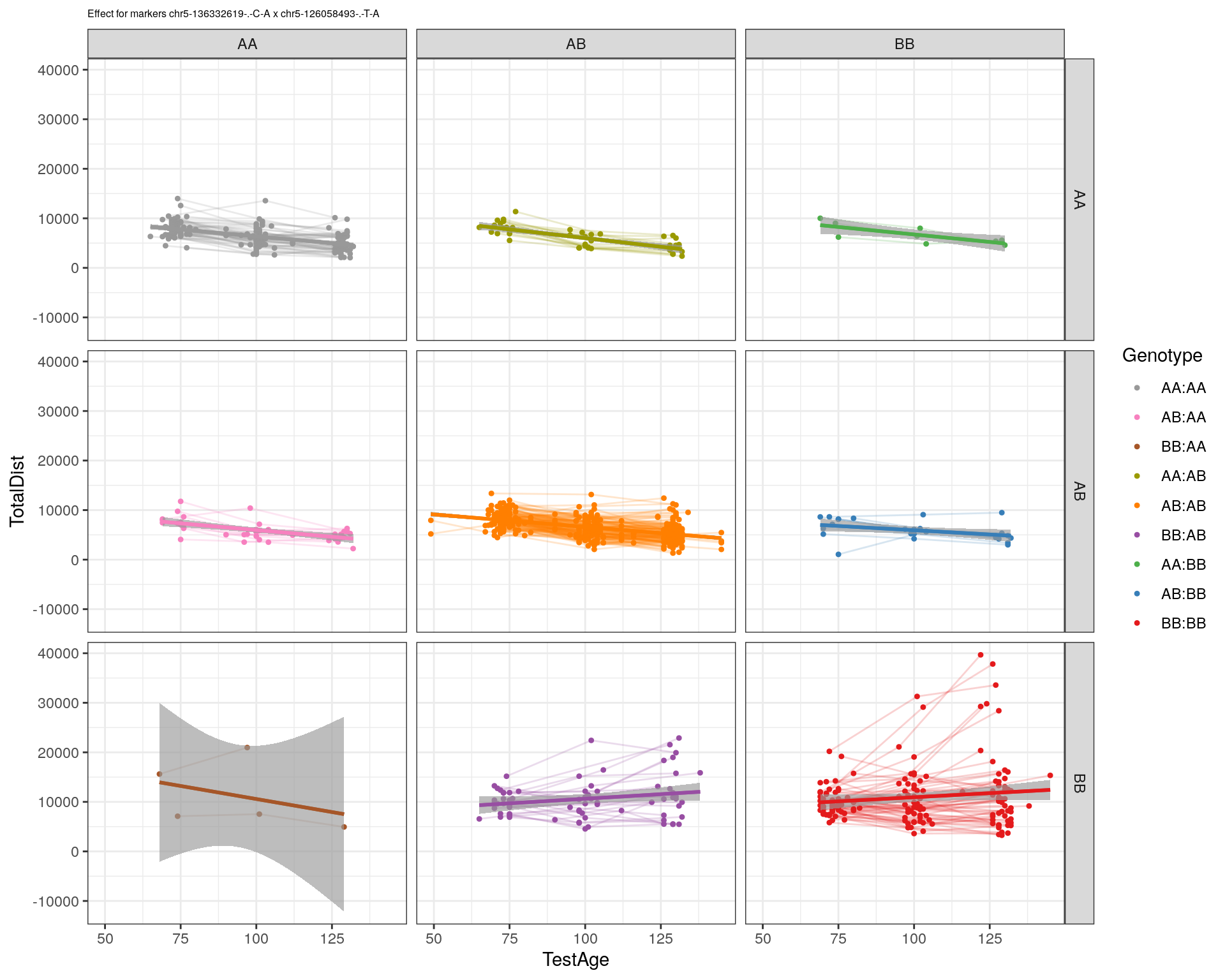
[1] "chr5-126551890-.-T-A"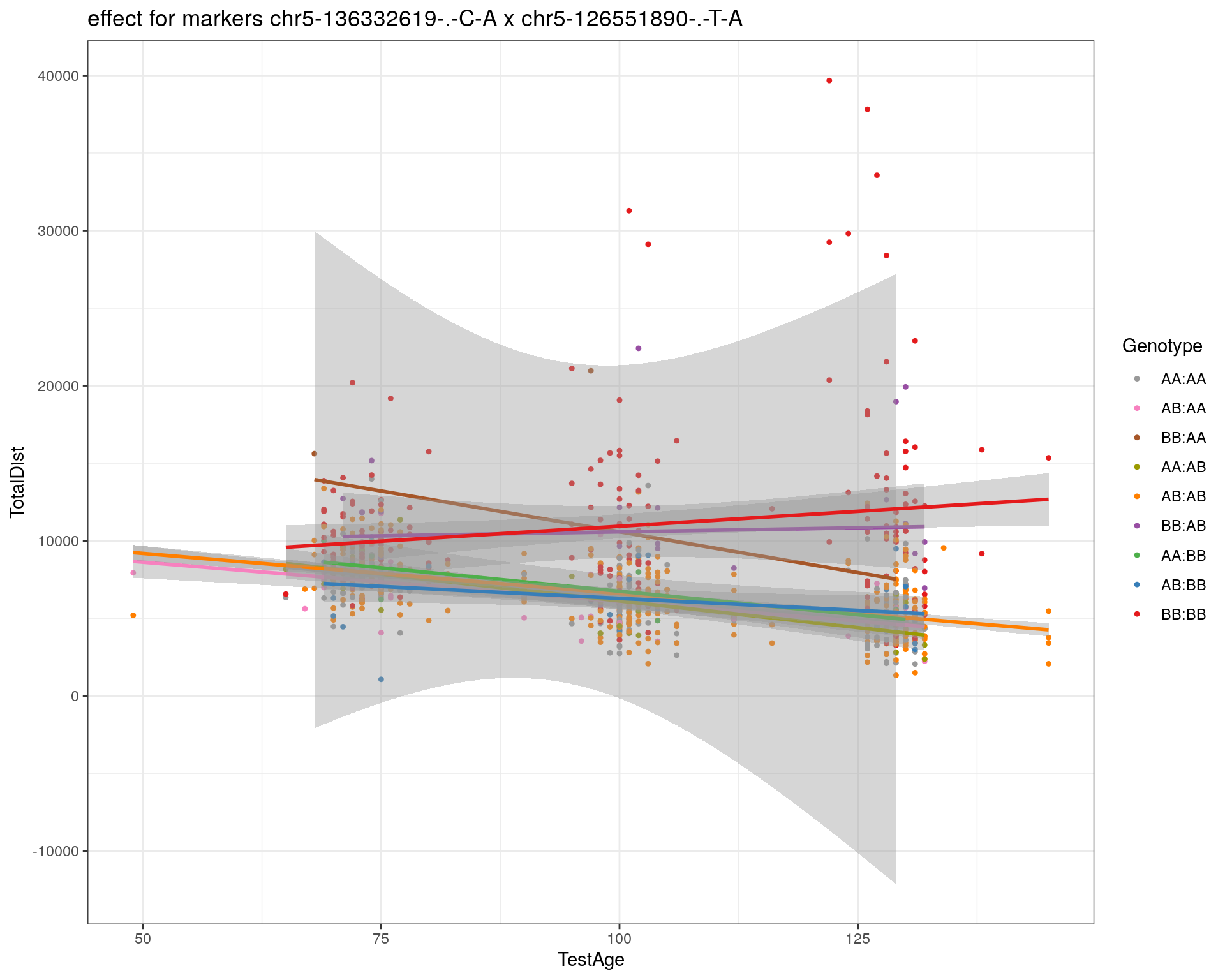
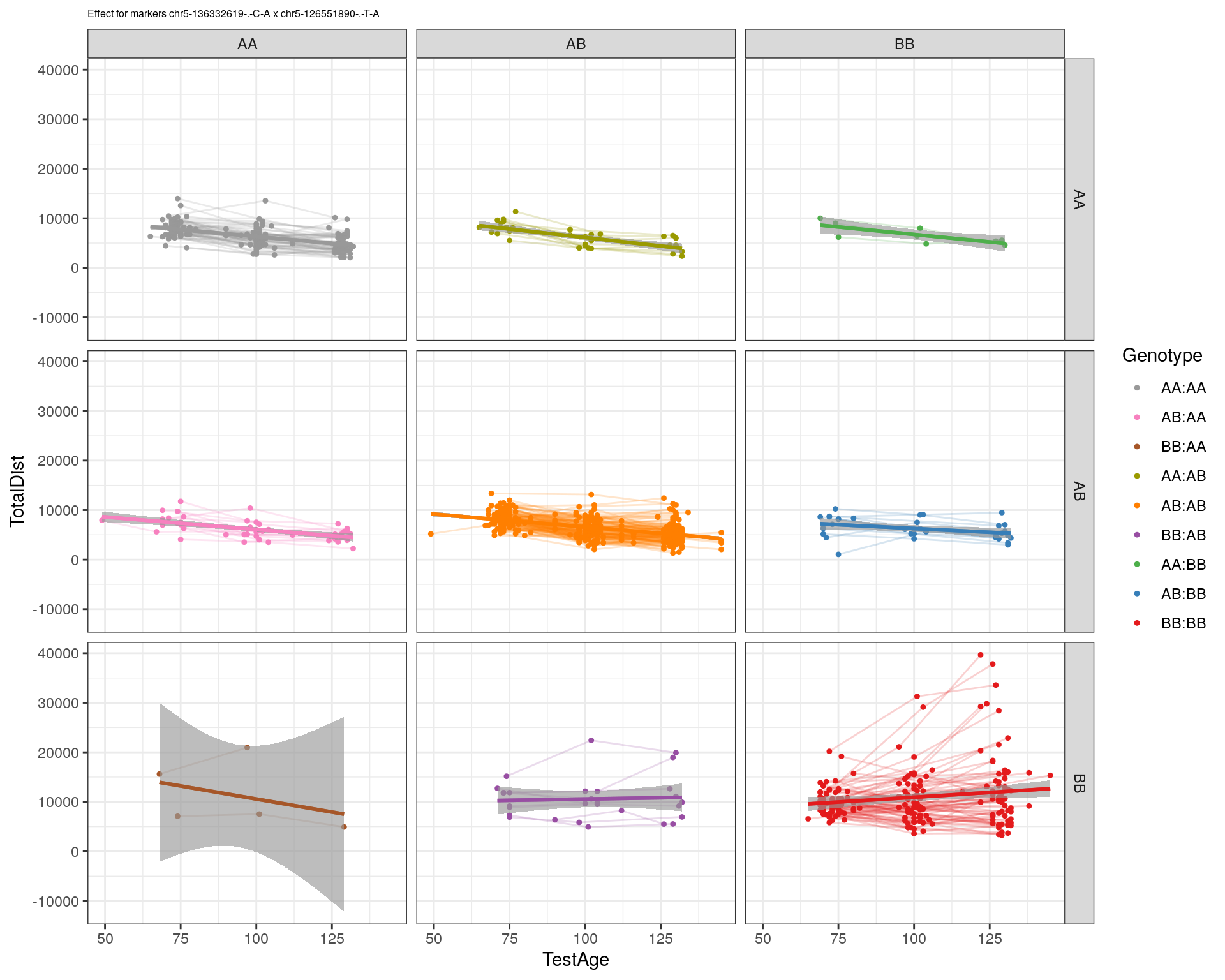
[1] "chr5-127565504-.-T-A"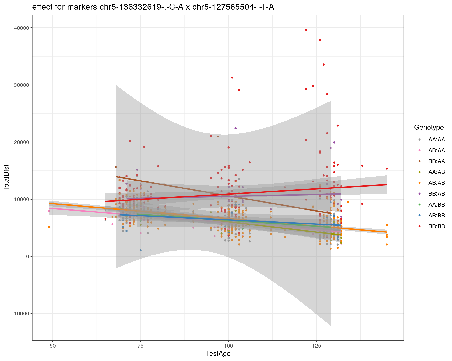
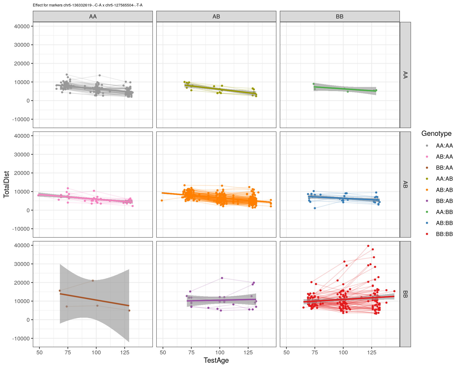
[1] "chr5-130394596-.-T-C"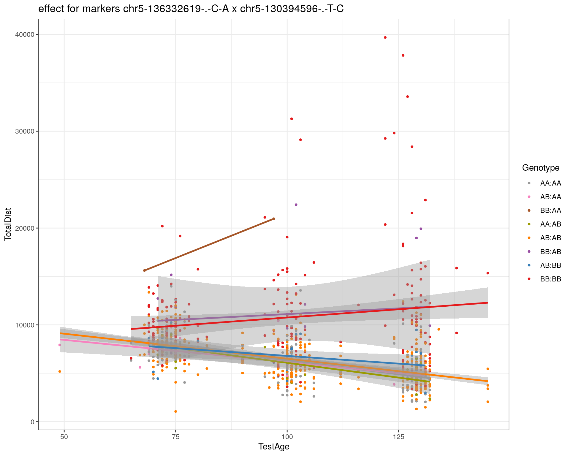
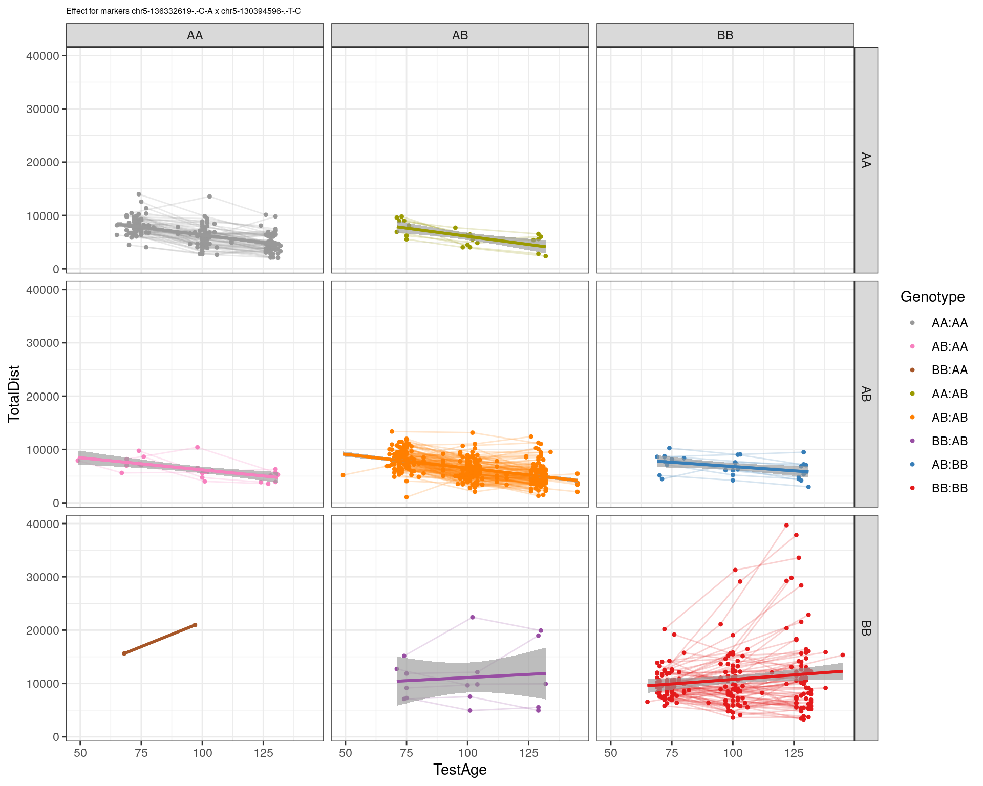
[1] "chr5-130943677-.-T-A"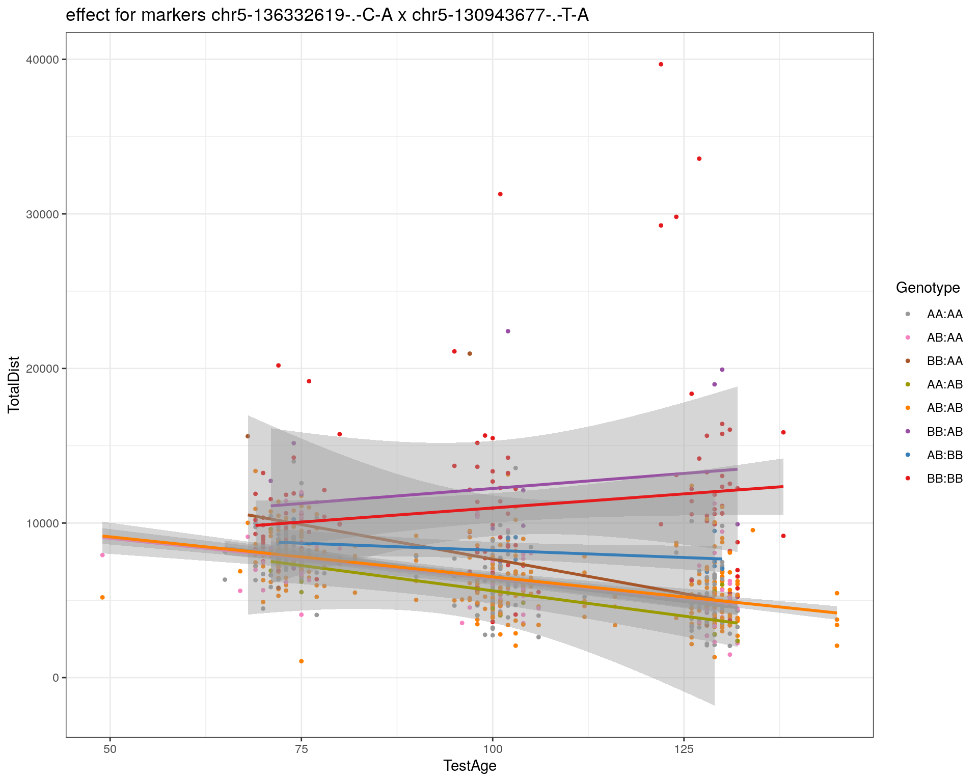
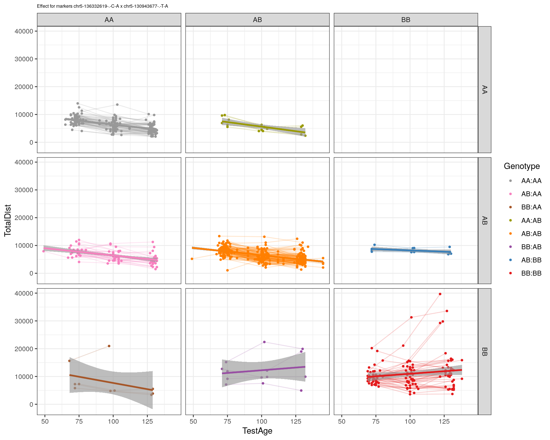
[1] "chr5-131298836-.-T-C"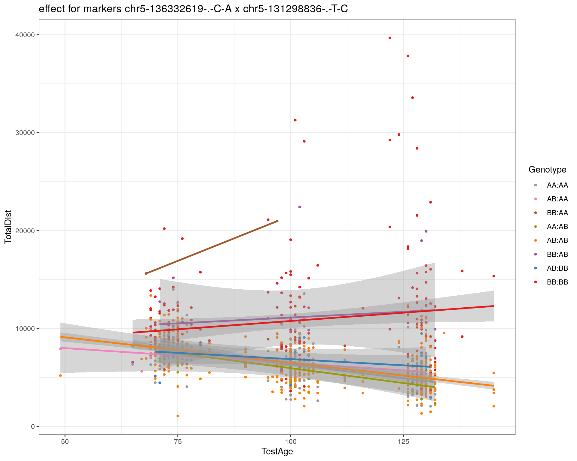
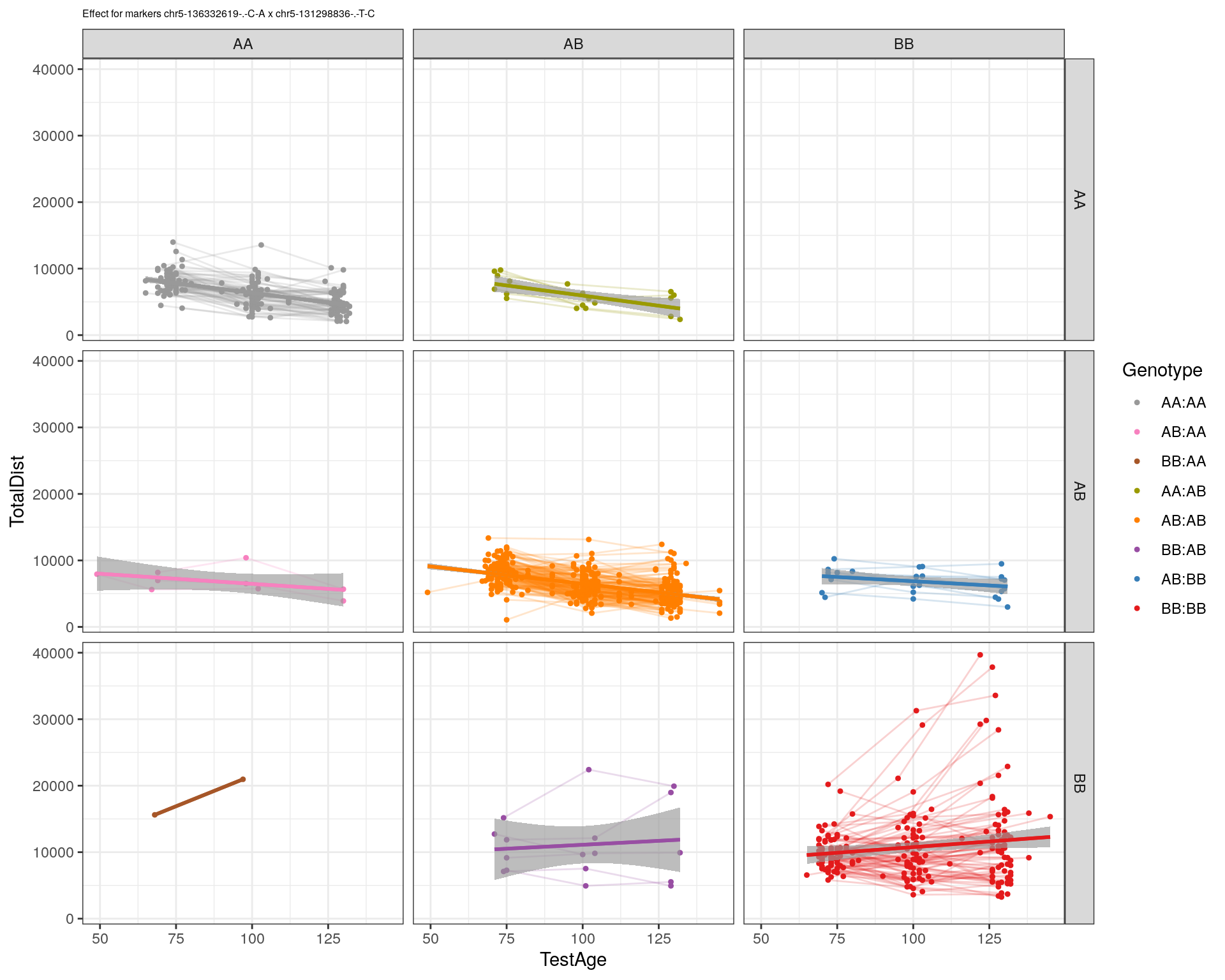
[1] "chr5-133052642-.-T-G"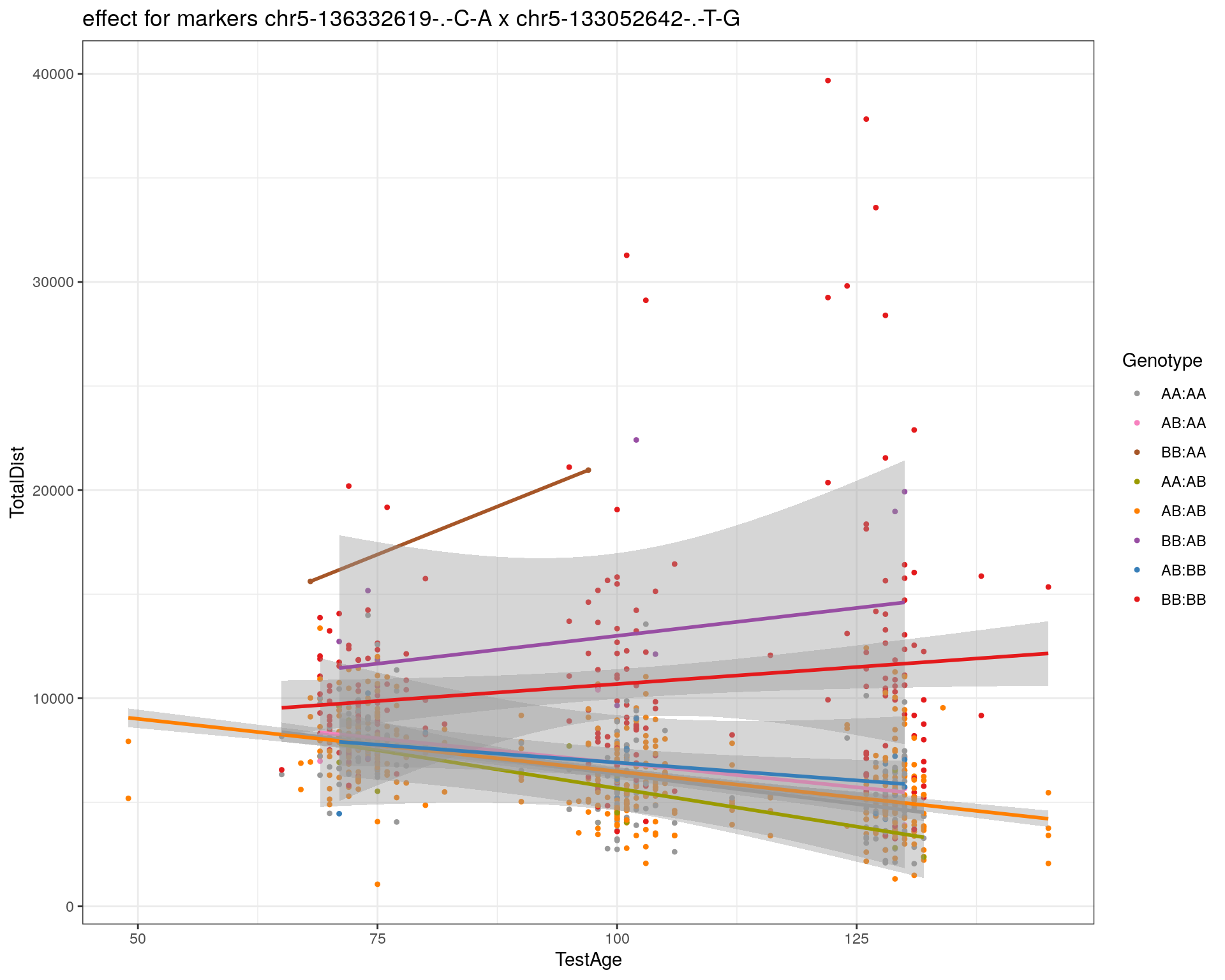
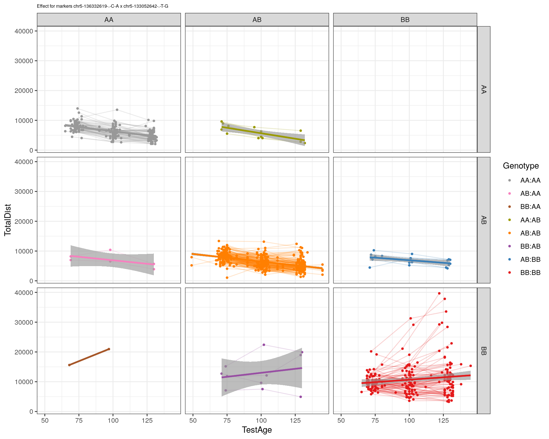
[1] "chr5-135960983-.-T-C"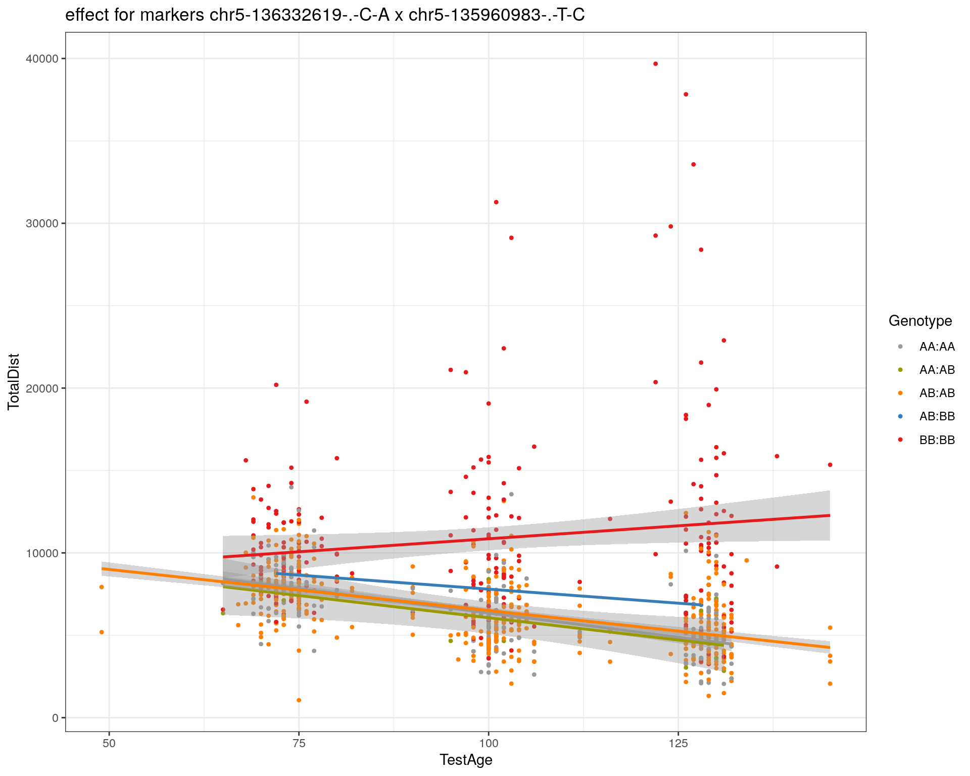
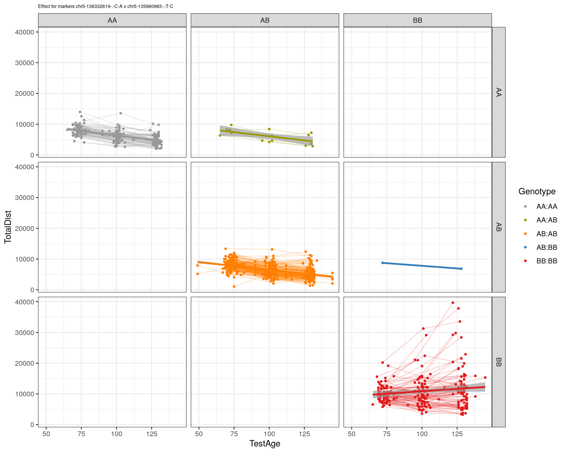
[1] "chr5-136332619-.-C-A"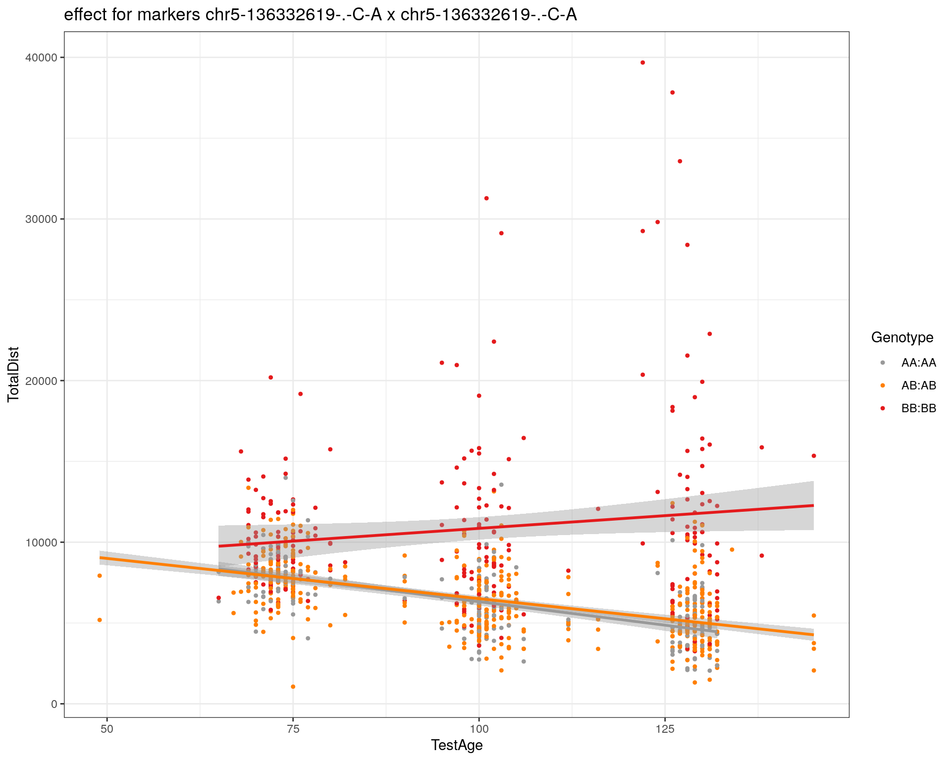
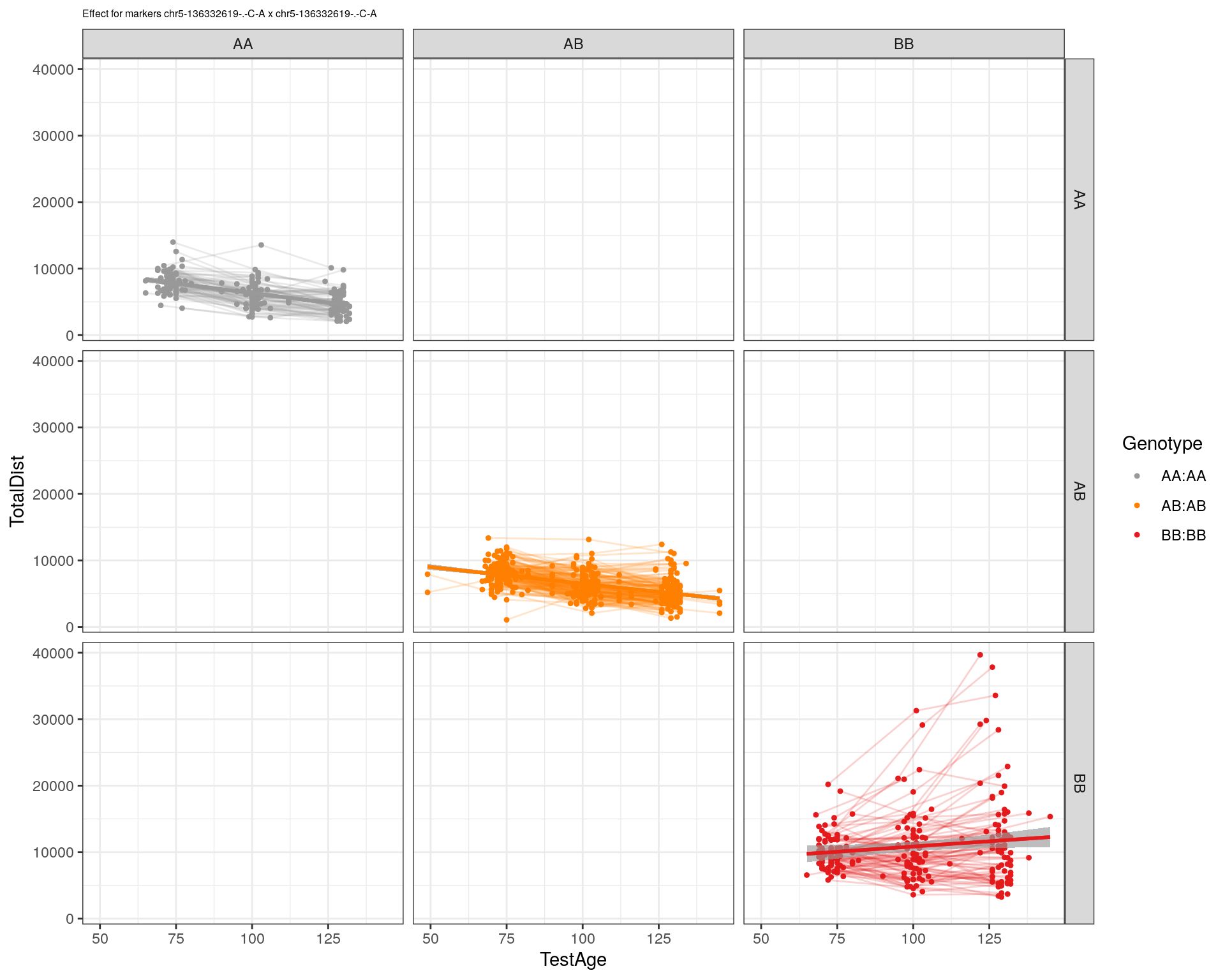
[1] "chr5-136844385-.-T-G"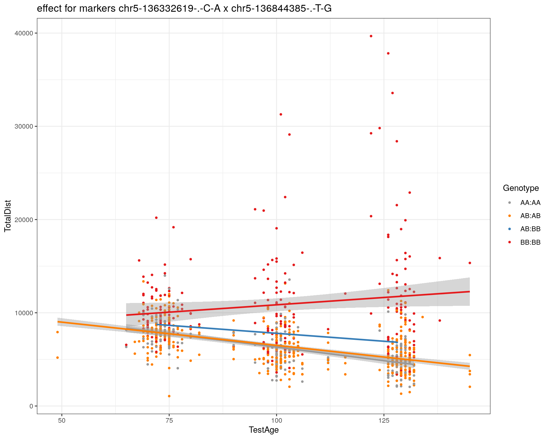
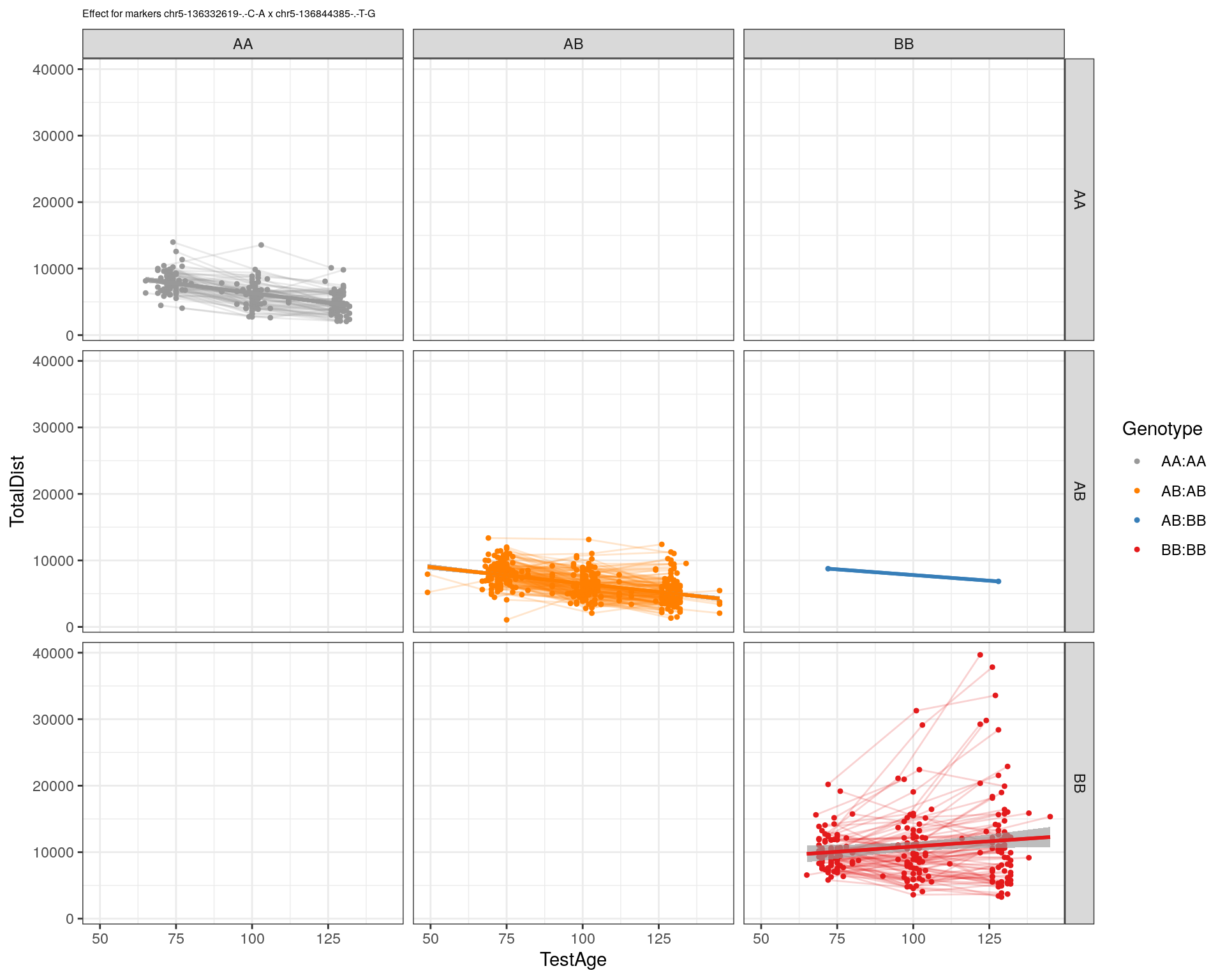
[1] "chr5-138956439-.-T-C"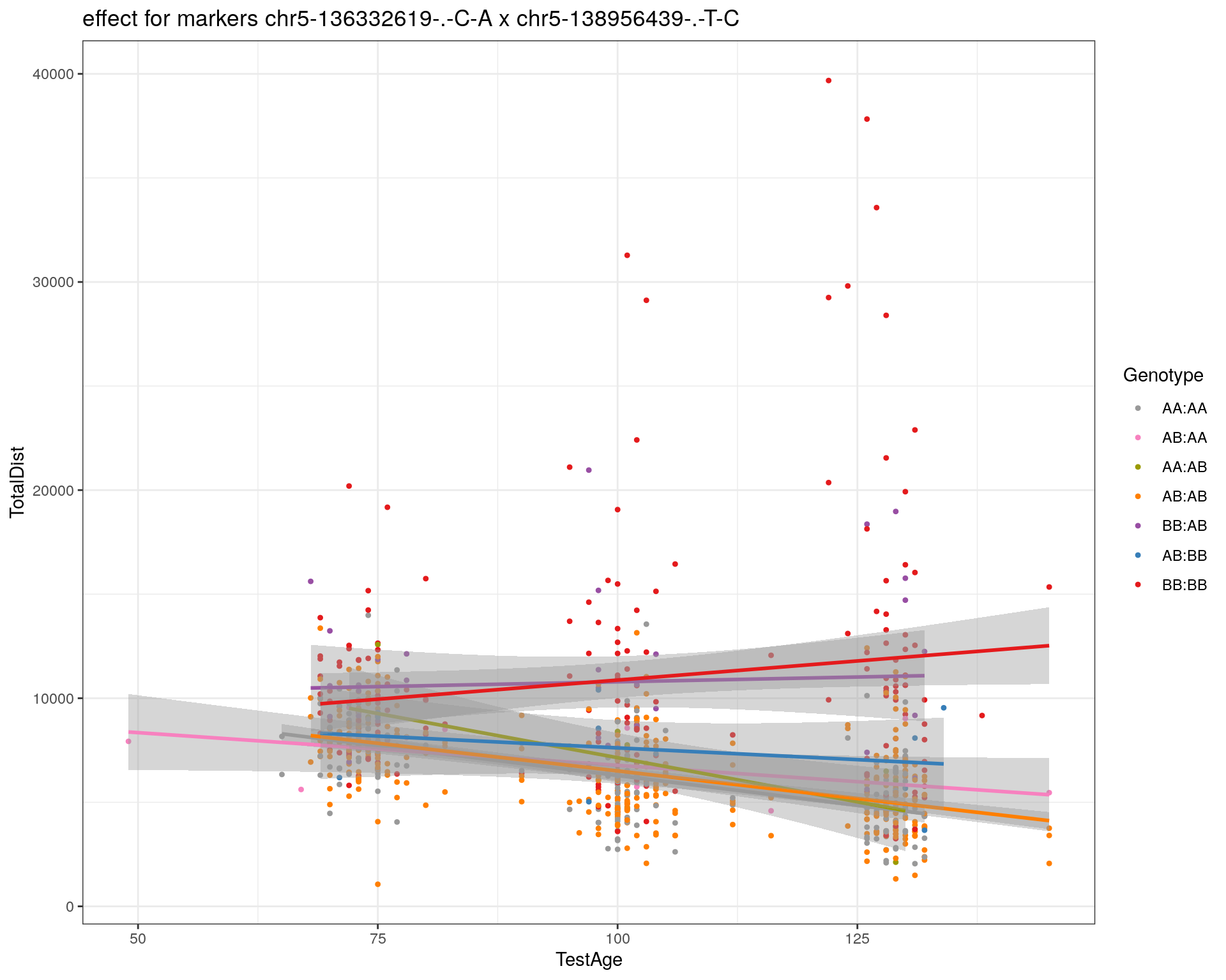
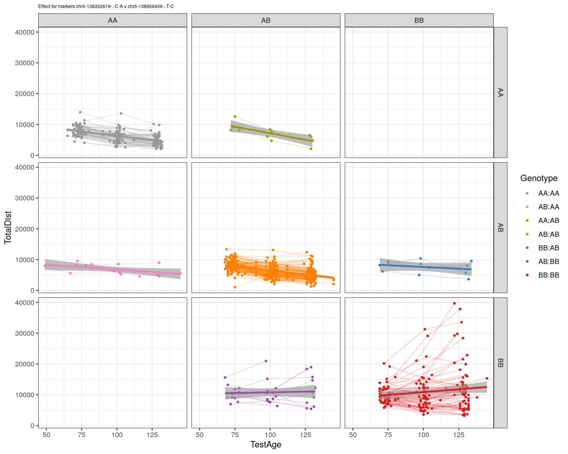
[1] "chr5-139706036-.-T-C"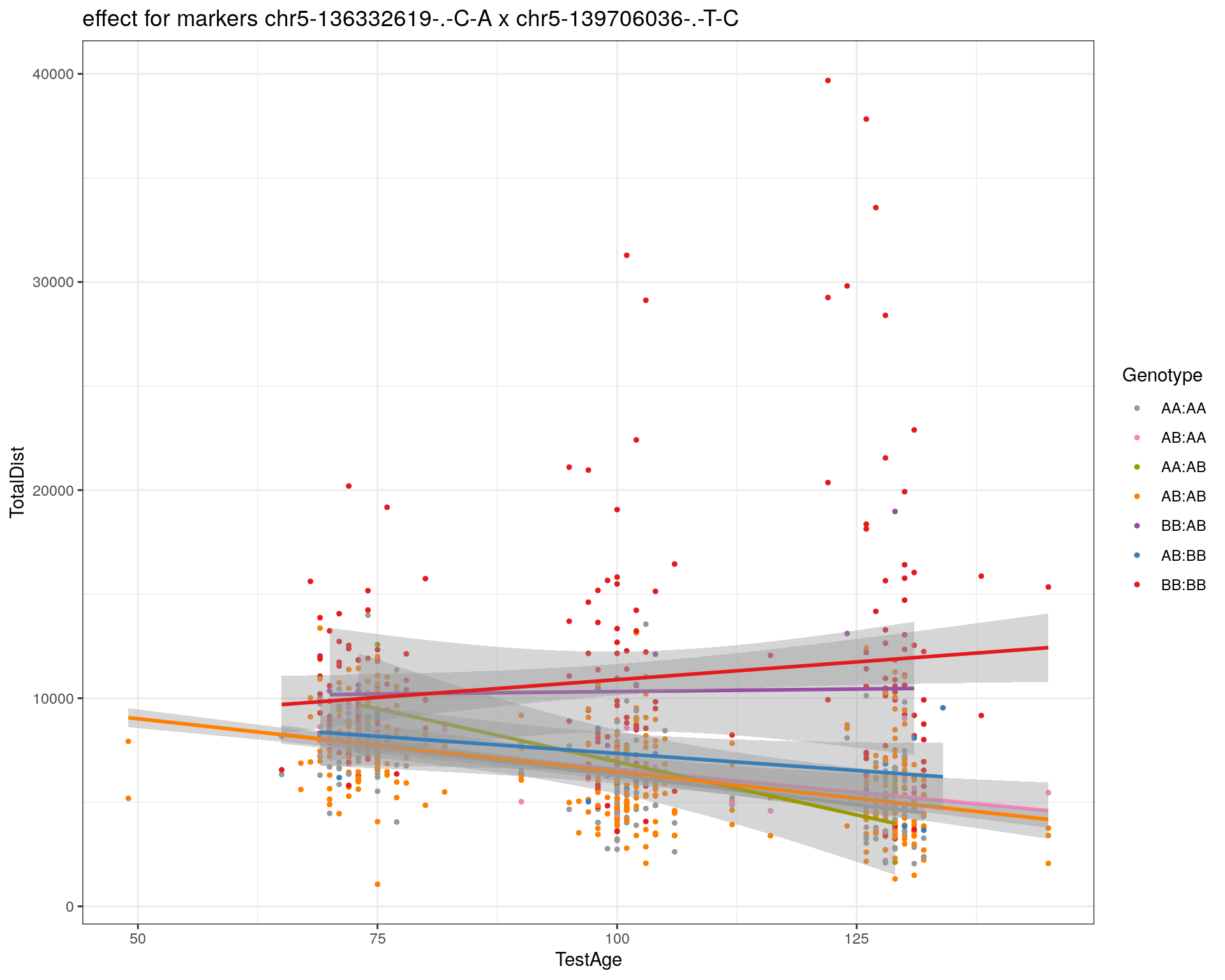
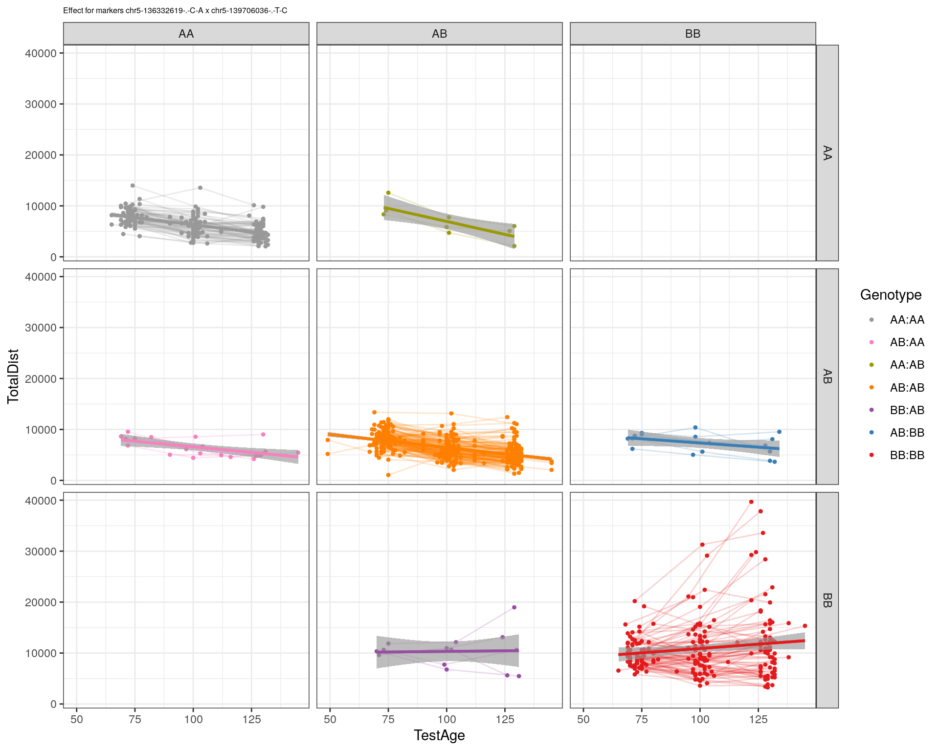
[1] "chr5-139891407-.-T-C"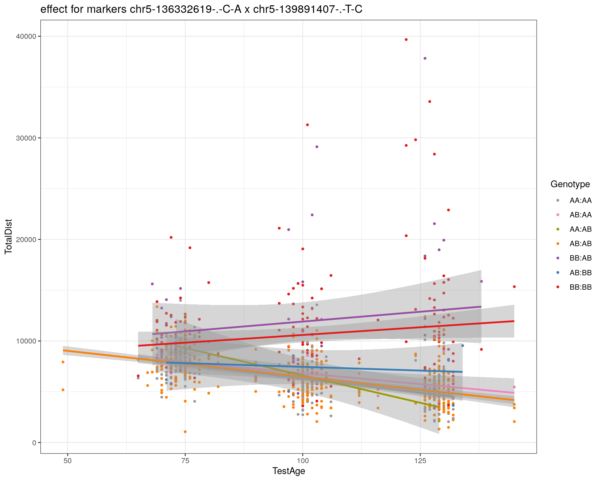
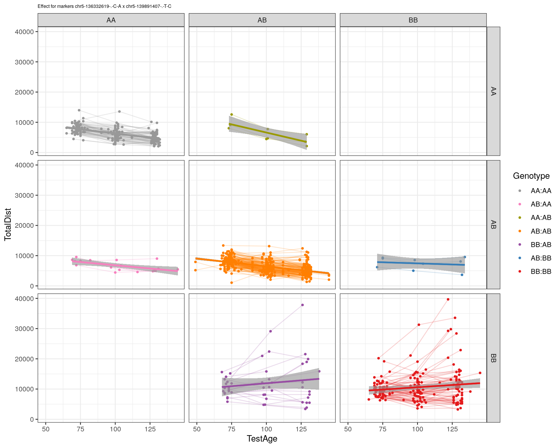
[1] "chr5-140071081-.-C-A"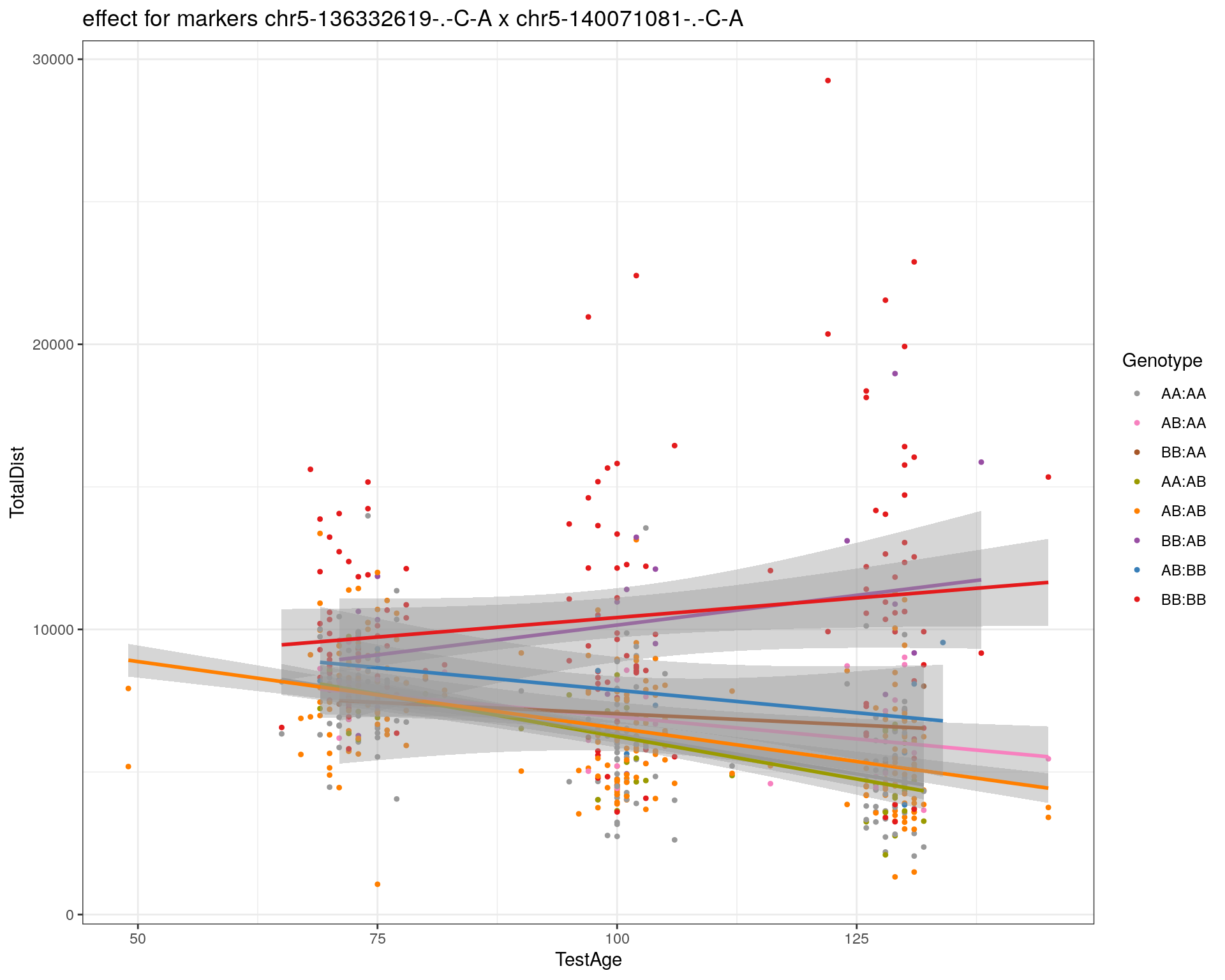
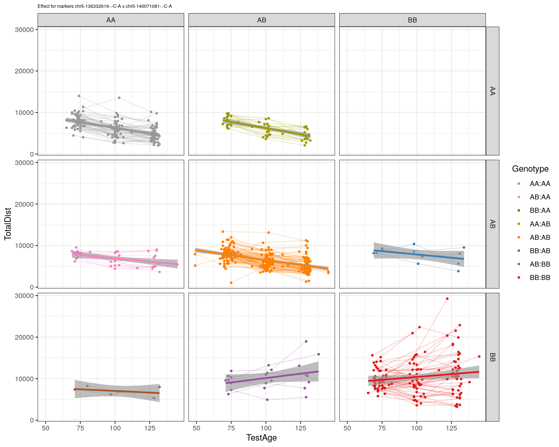
[1] "chr7-35061547-.-A-G"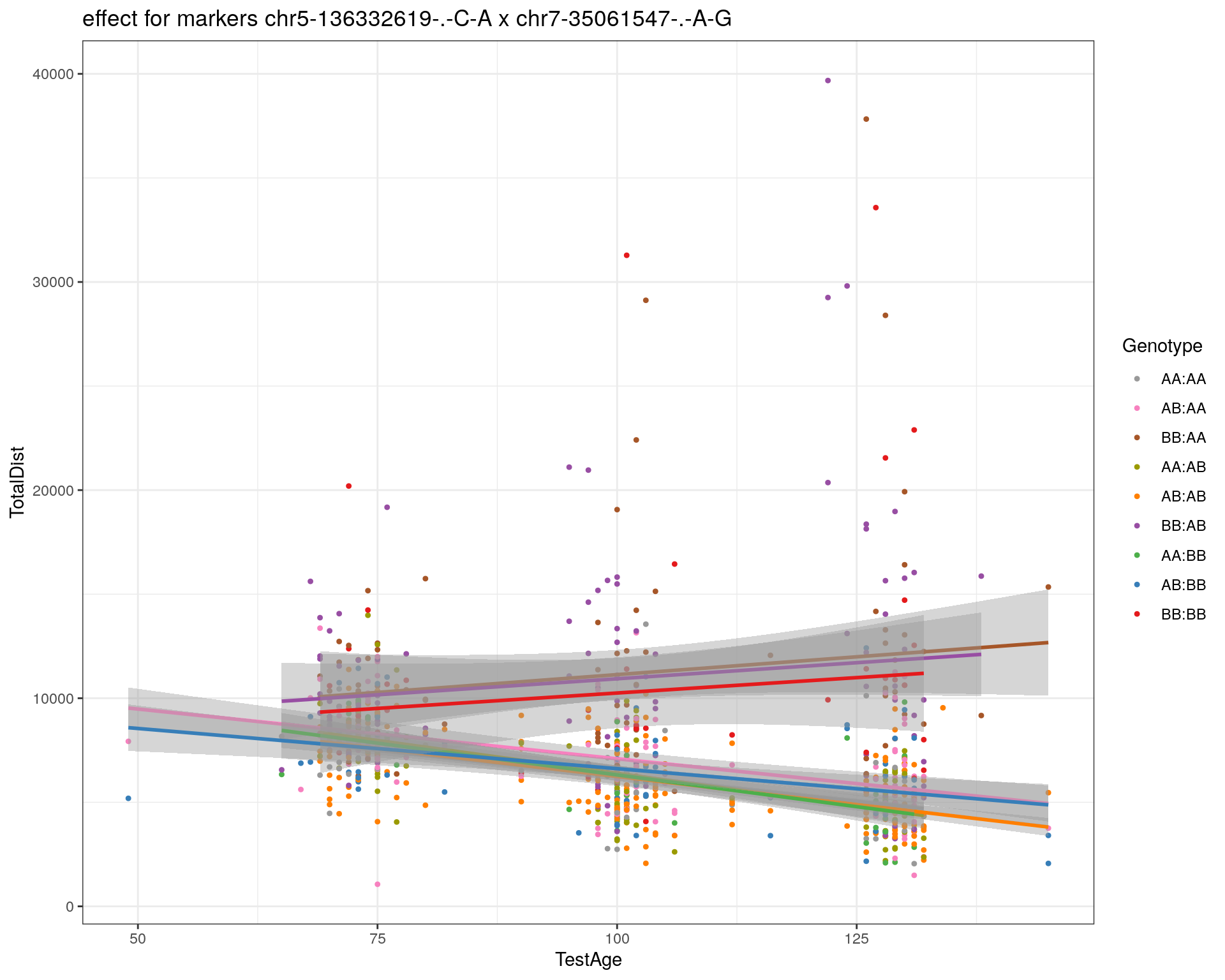
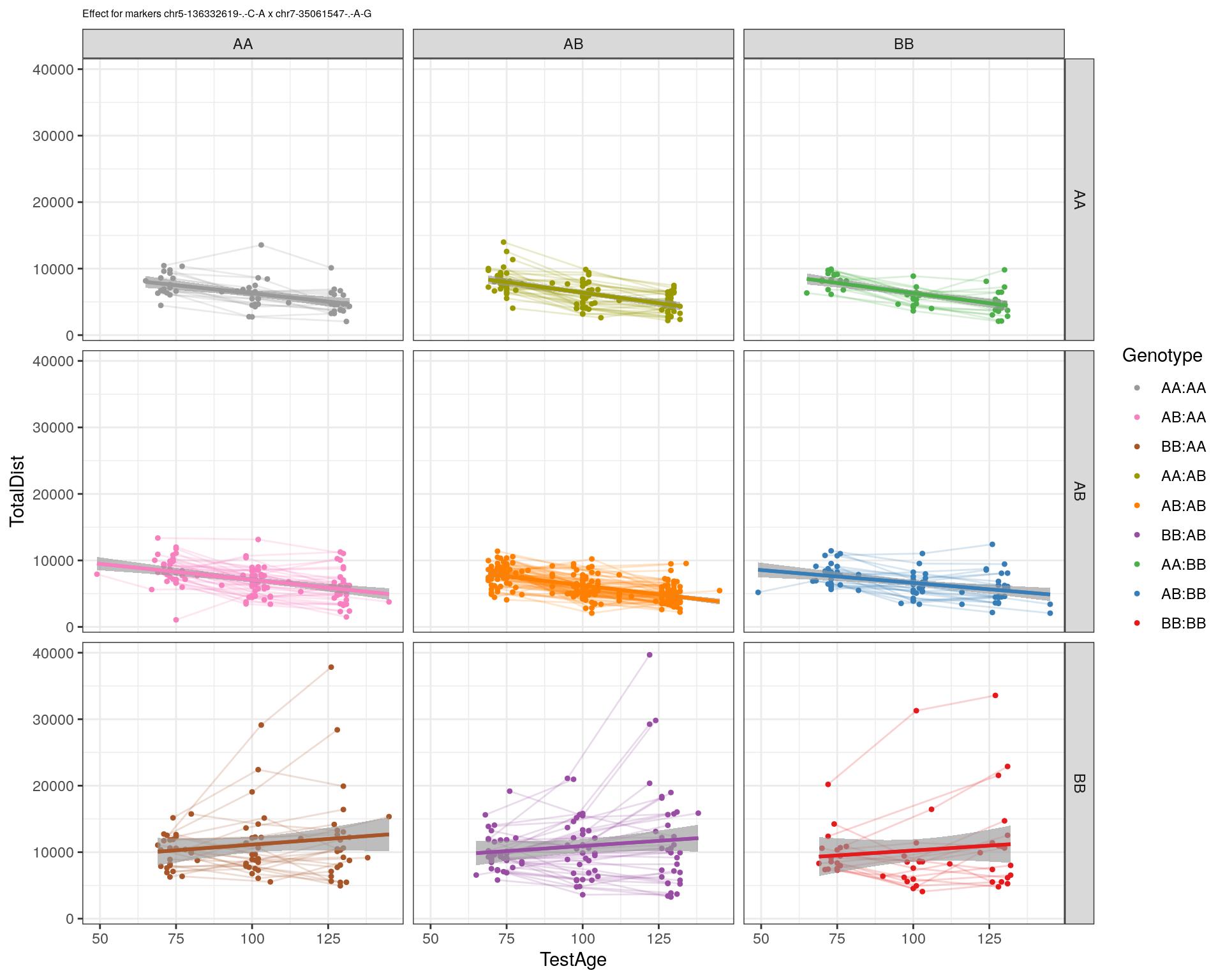
[1] "chr7-44272713-.-T-C"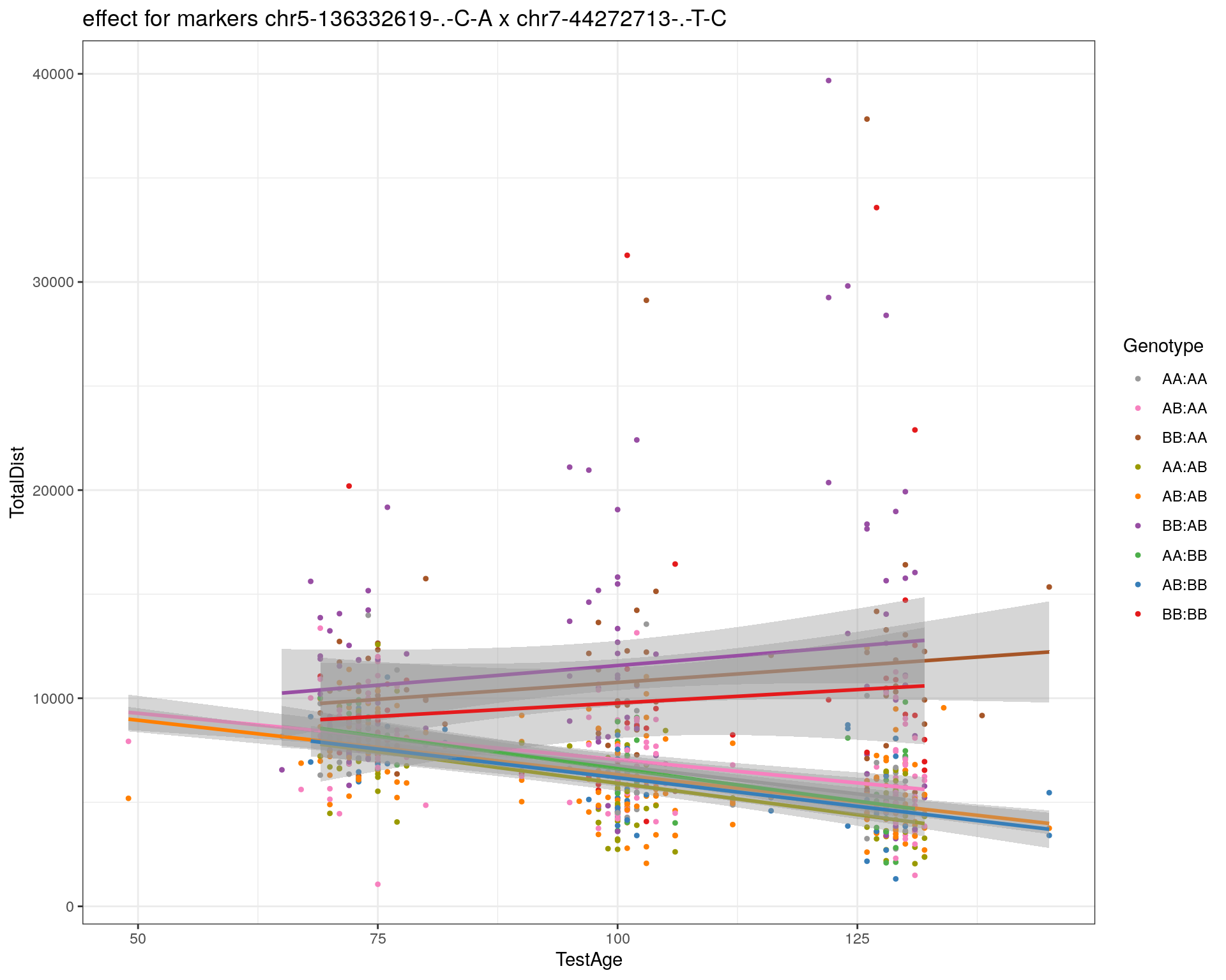
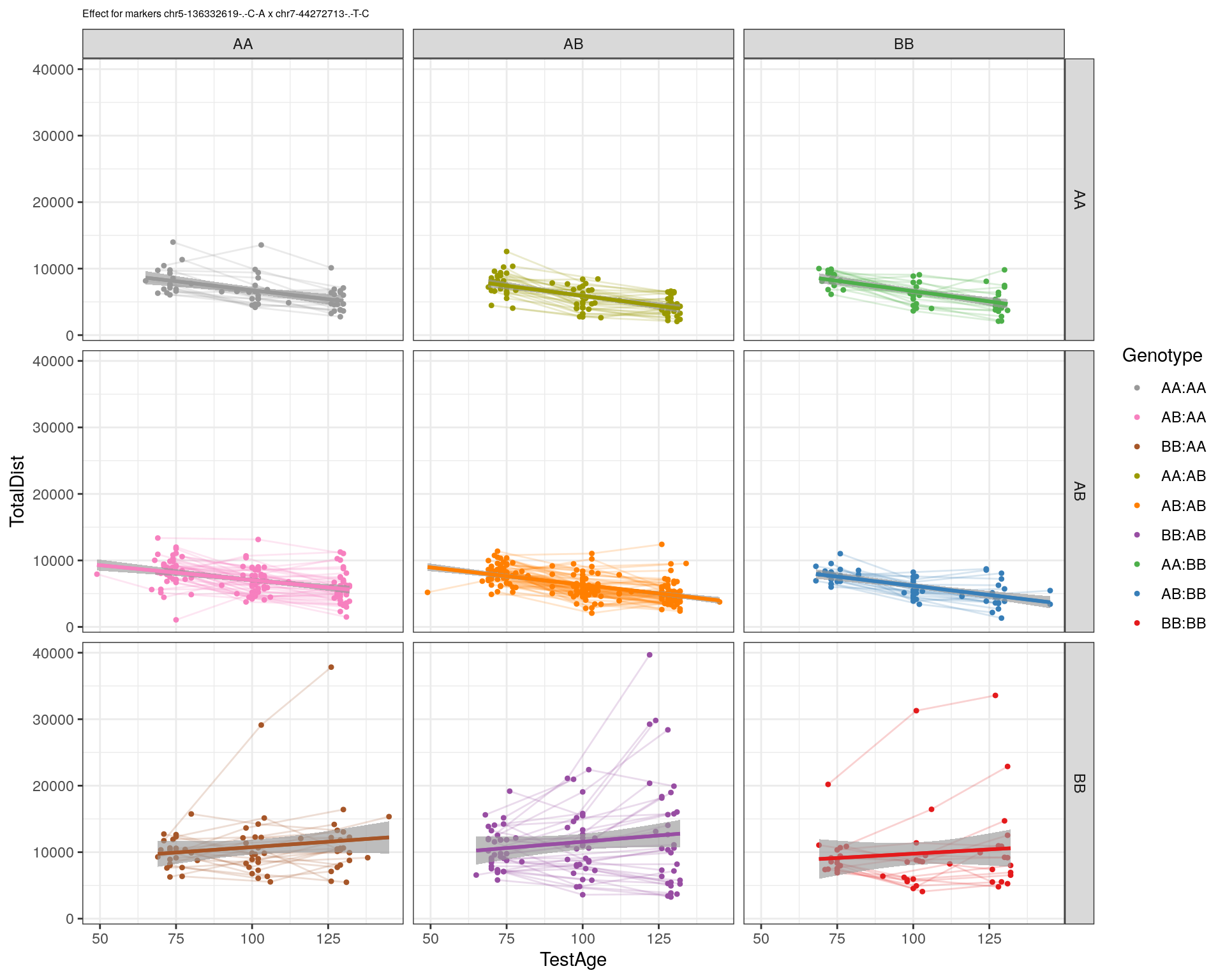
[1] "chr7-66785411-.-A-G"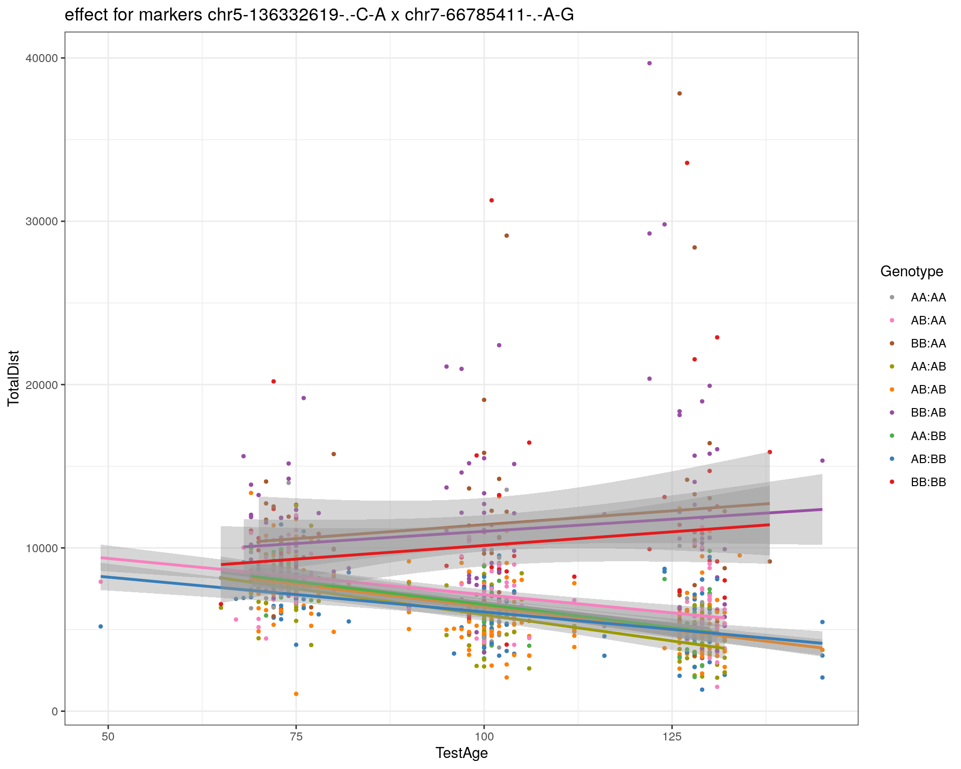
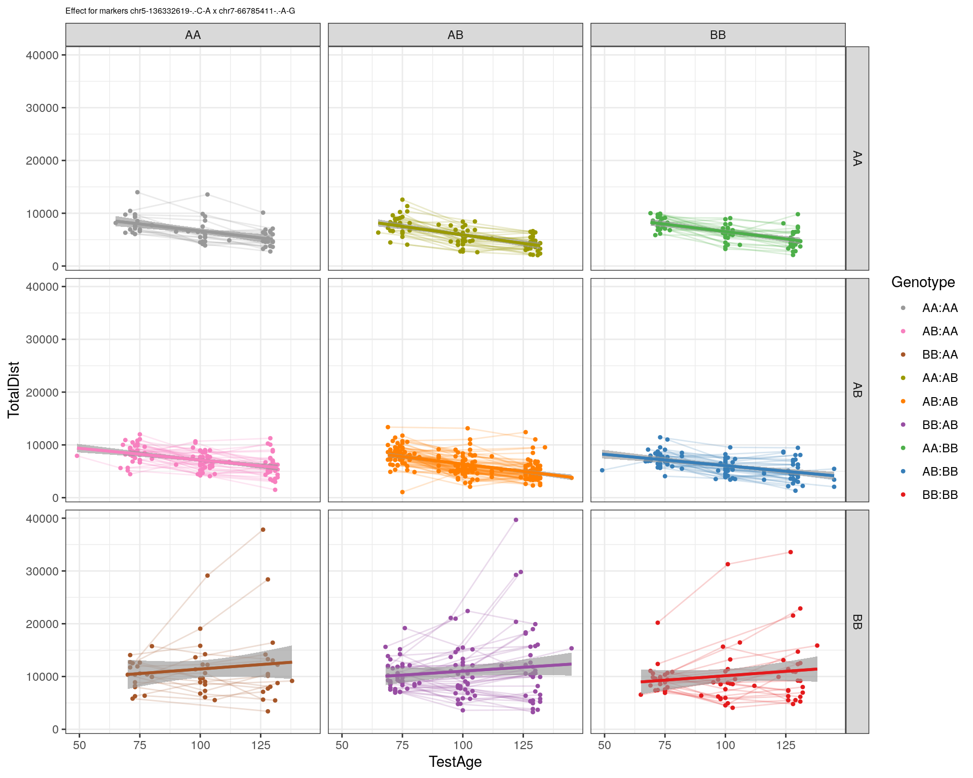
[1] "chr7-112510032-.-A-T"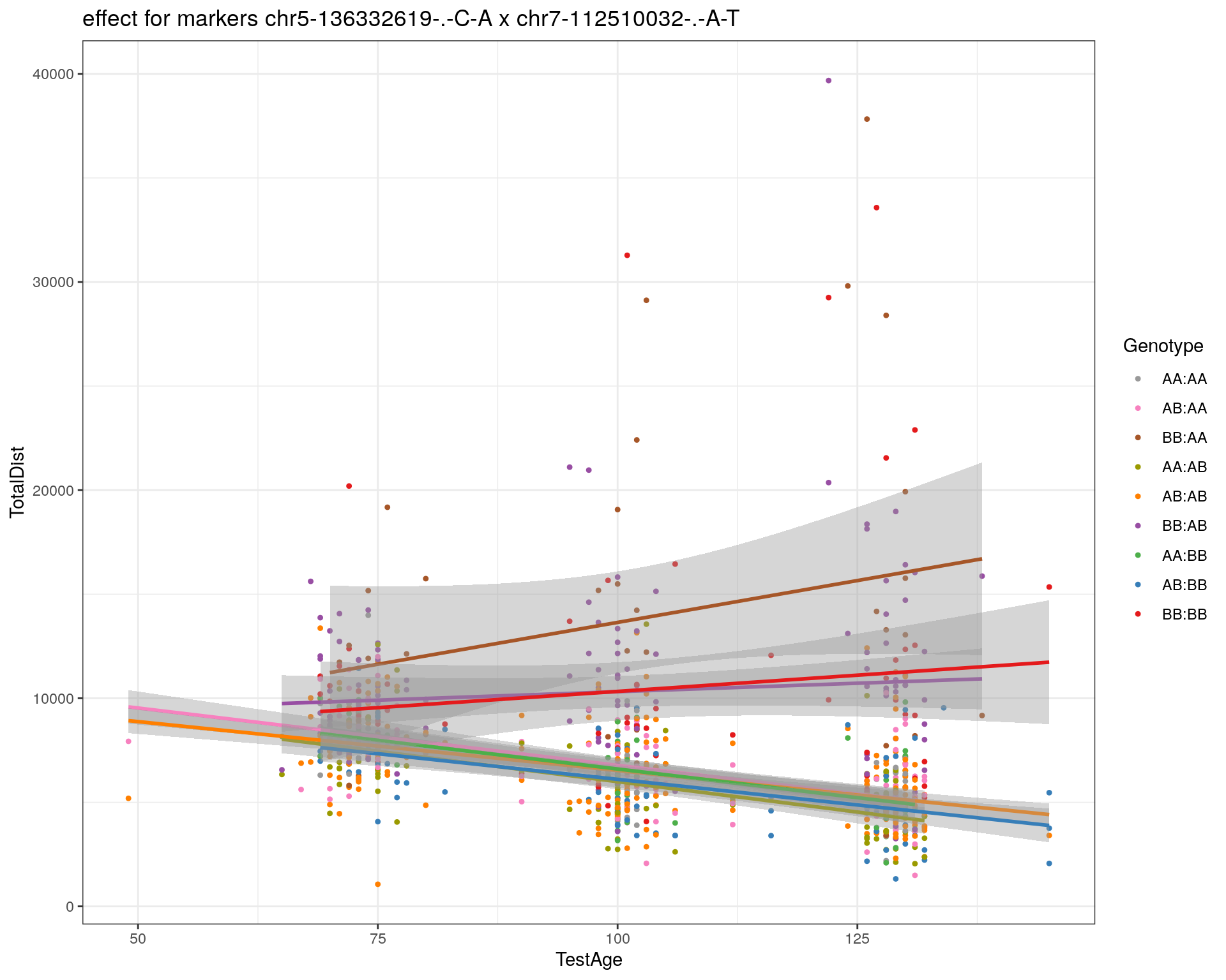
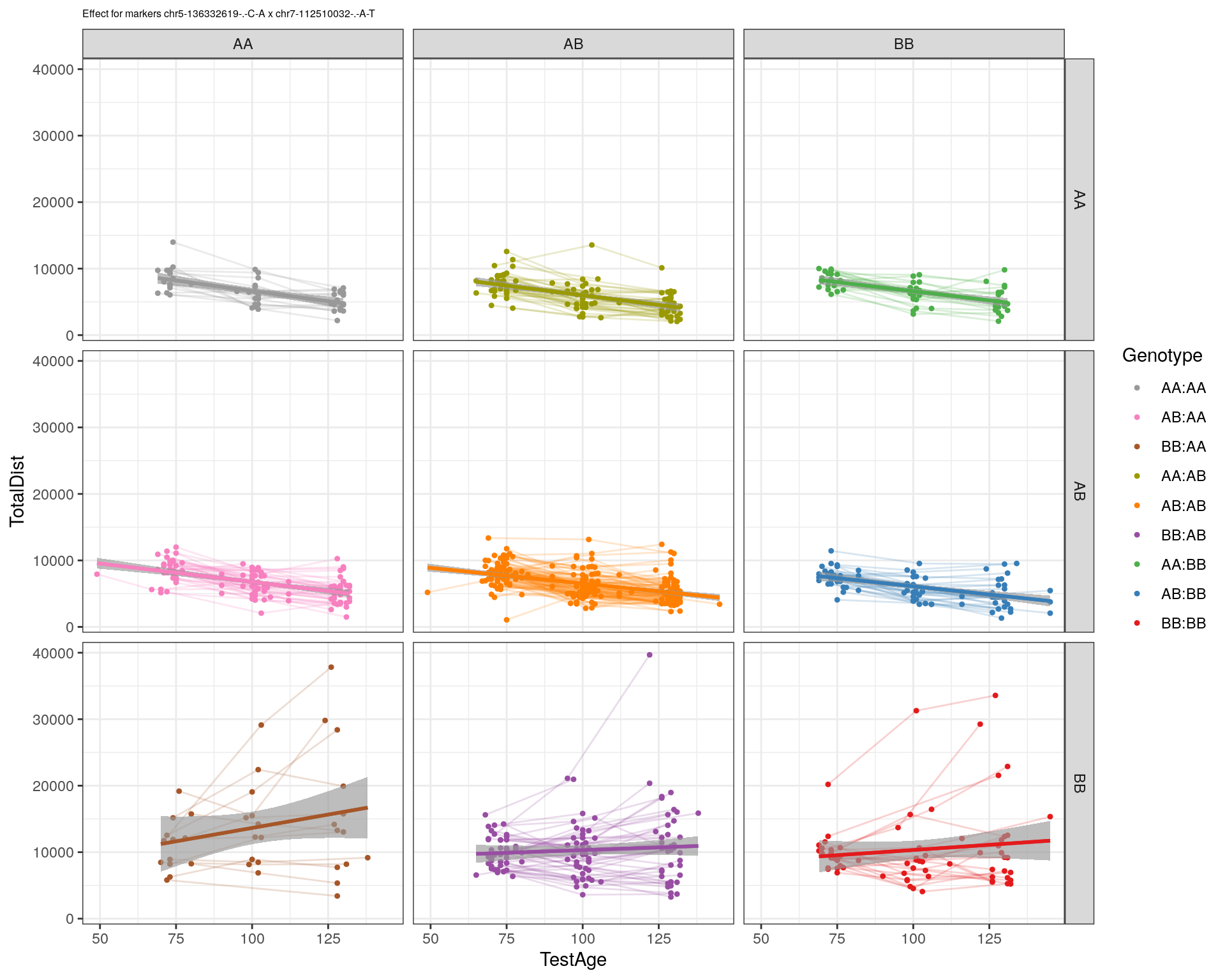
[1] "chr8-91986173-.-T-C"
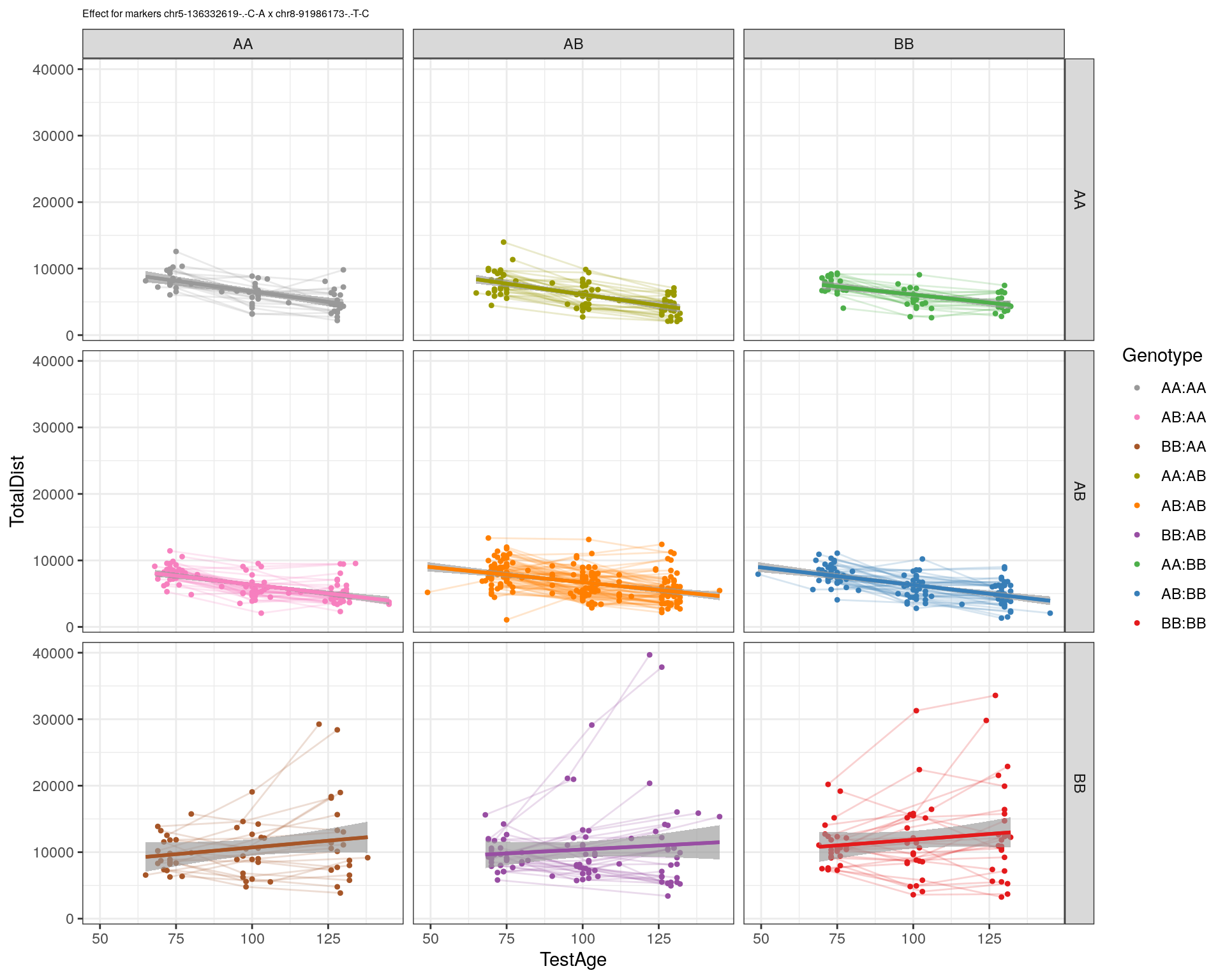
[1] "chr8-99395759-.-T-C"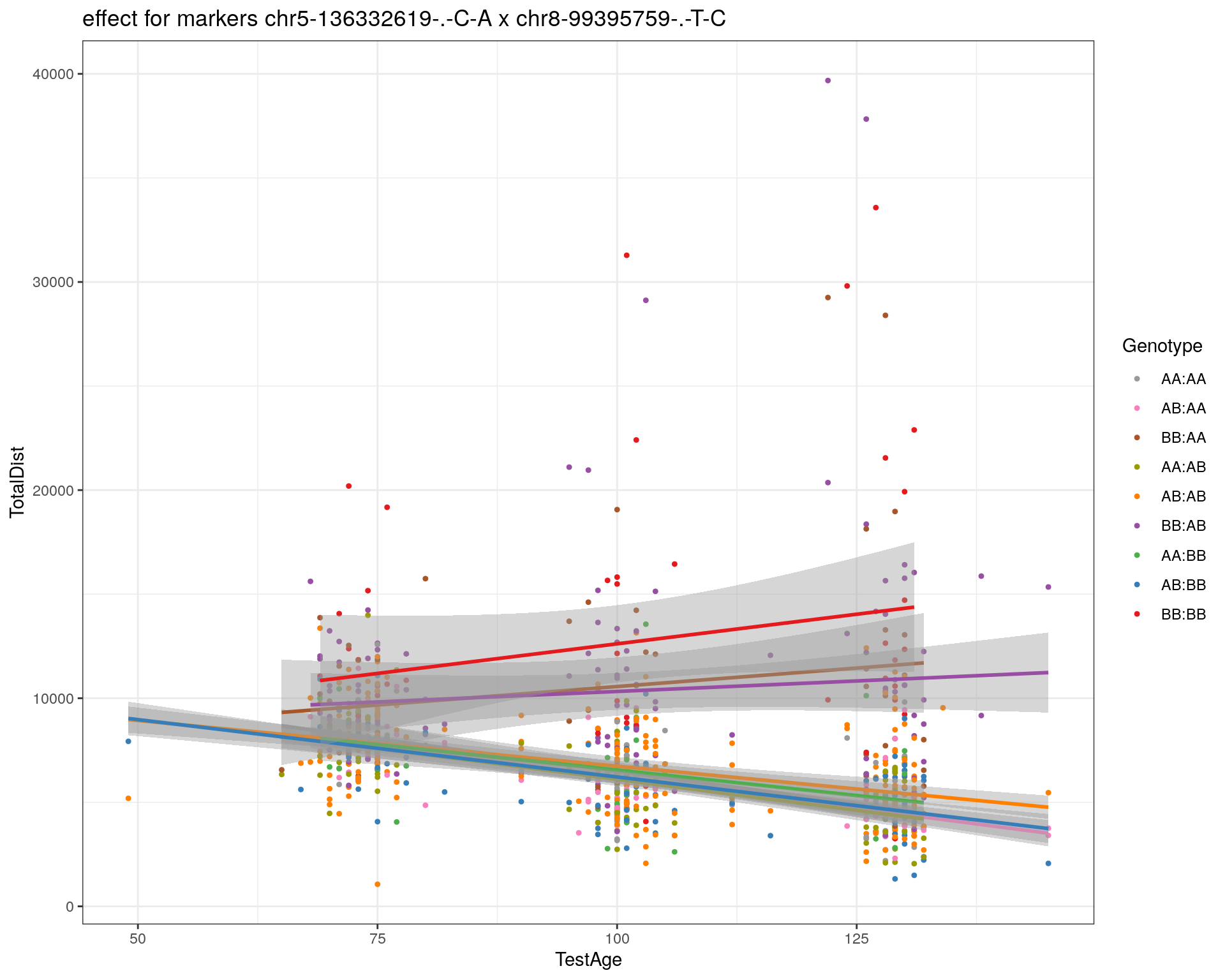
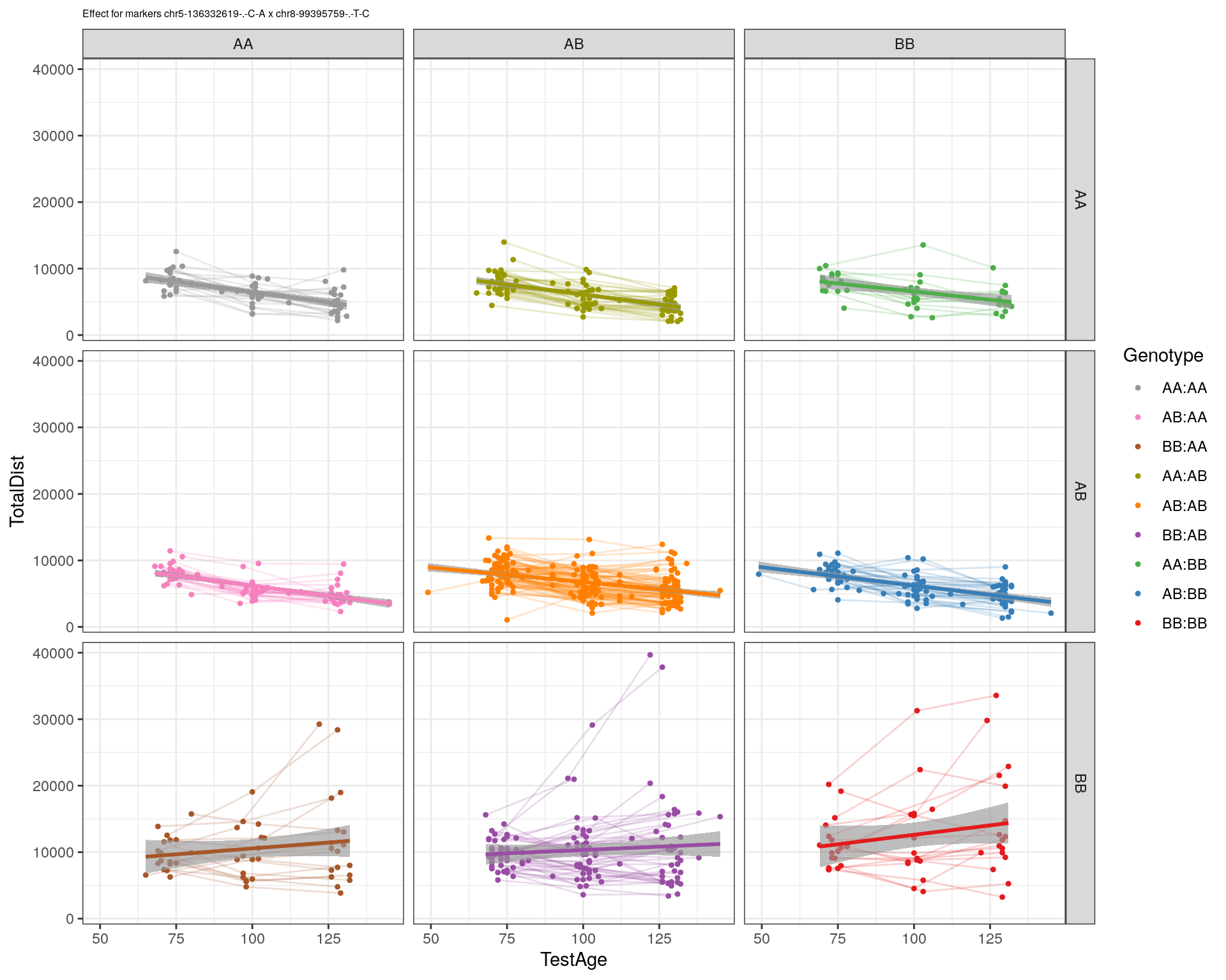
[1] "chr8-112465004-.-G-A"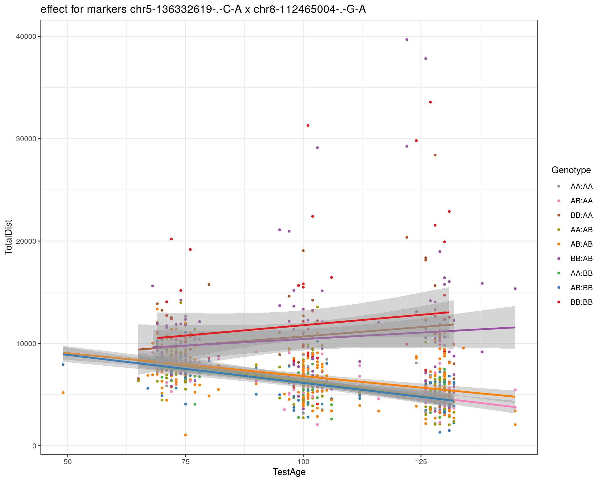
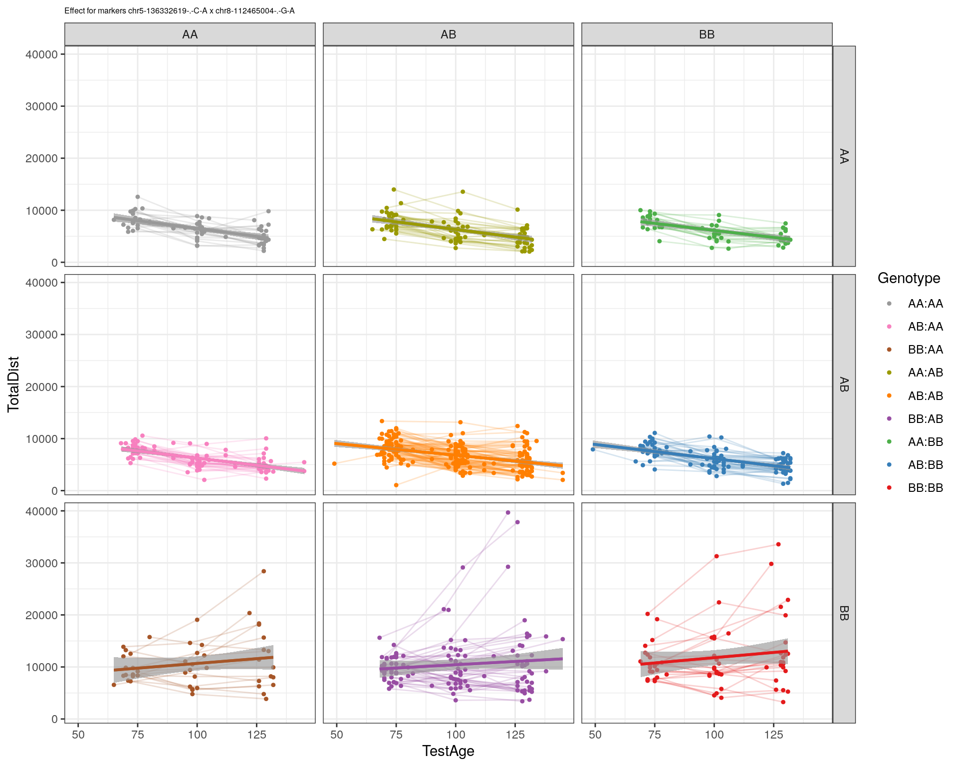
[1] "chr9-64698947-.-C-T"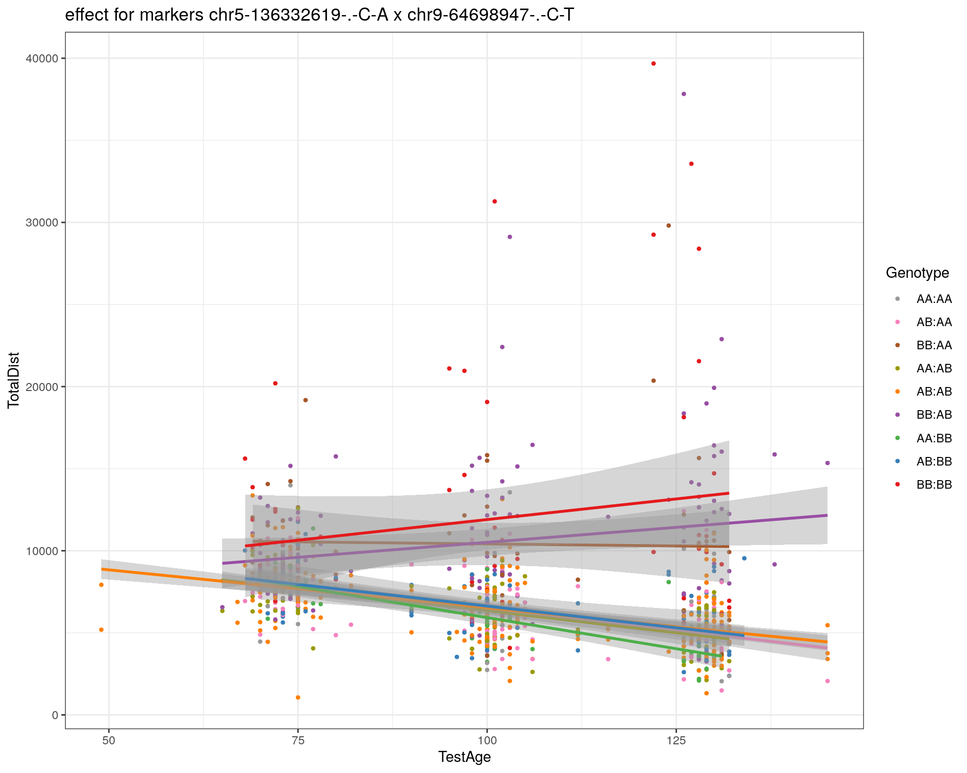

[1] "chr9-65857475-.-T-C"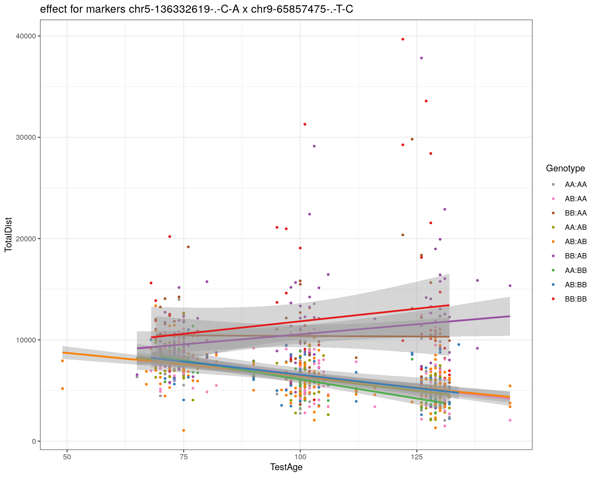
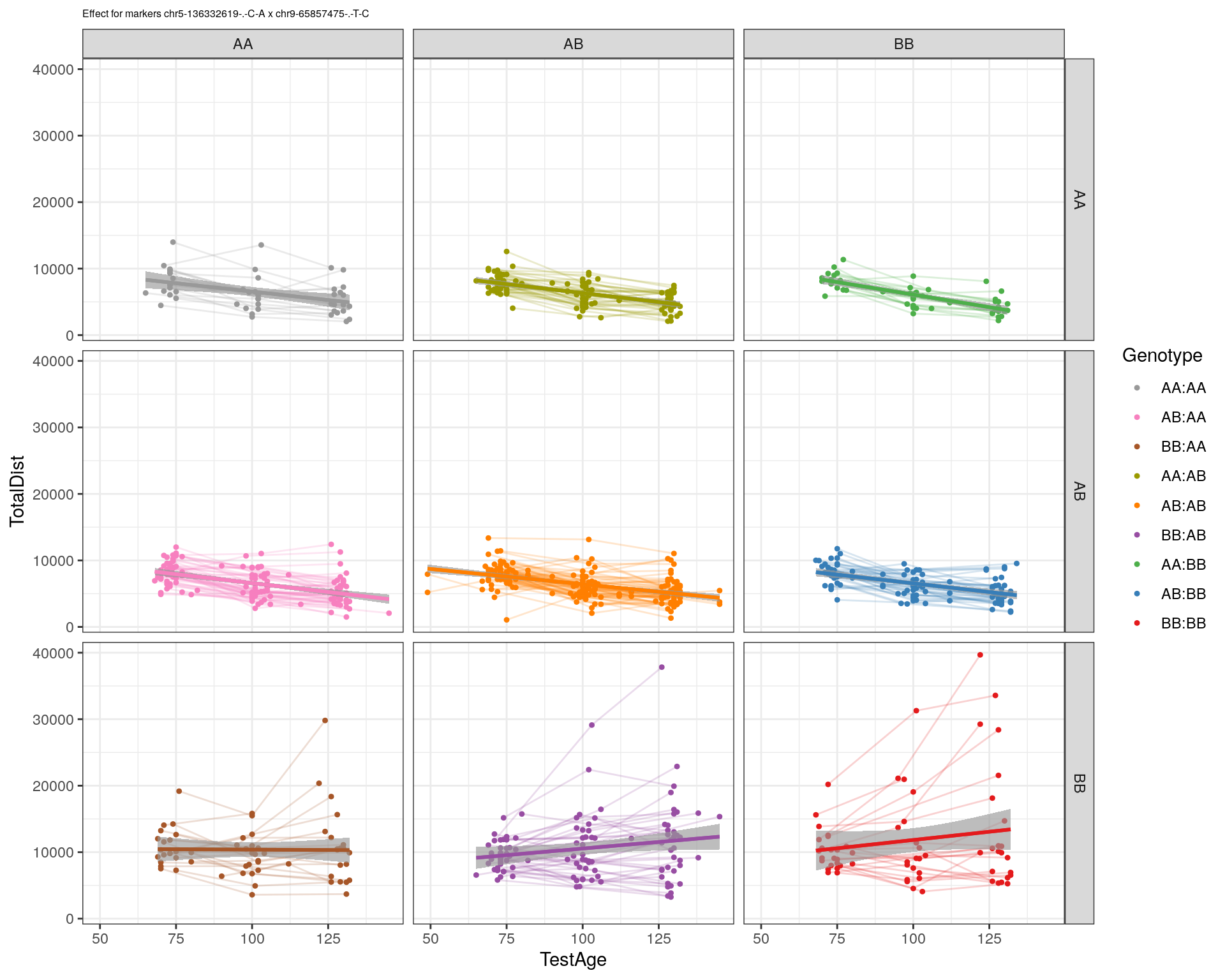
[1] "chr9-69415567-.-T-A"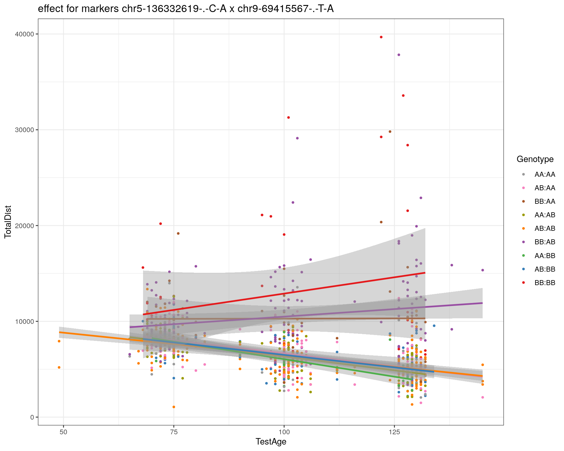
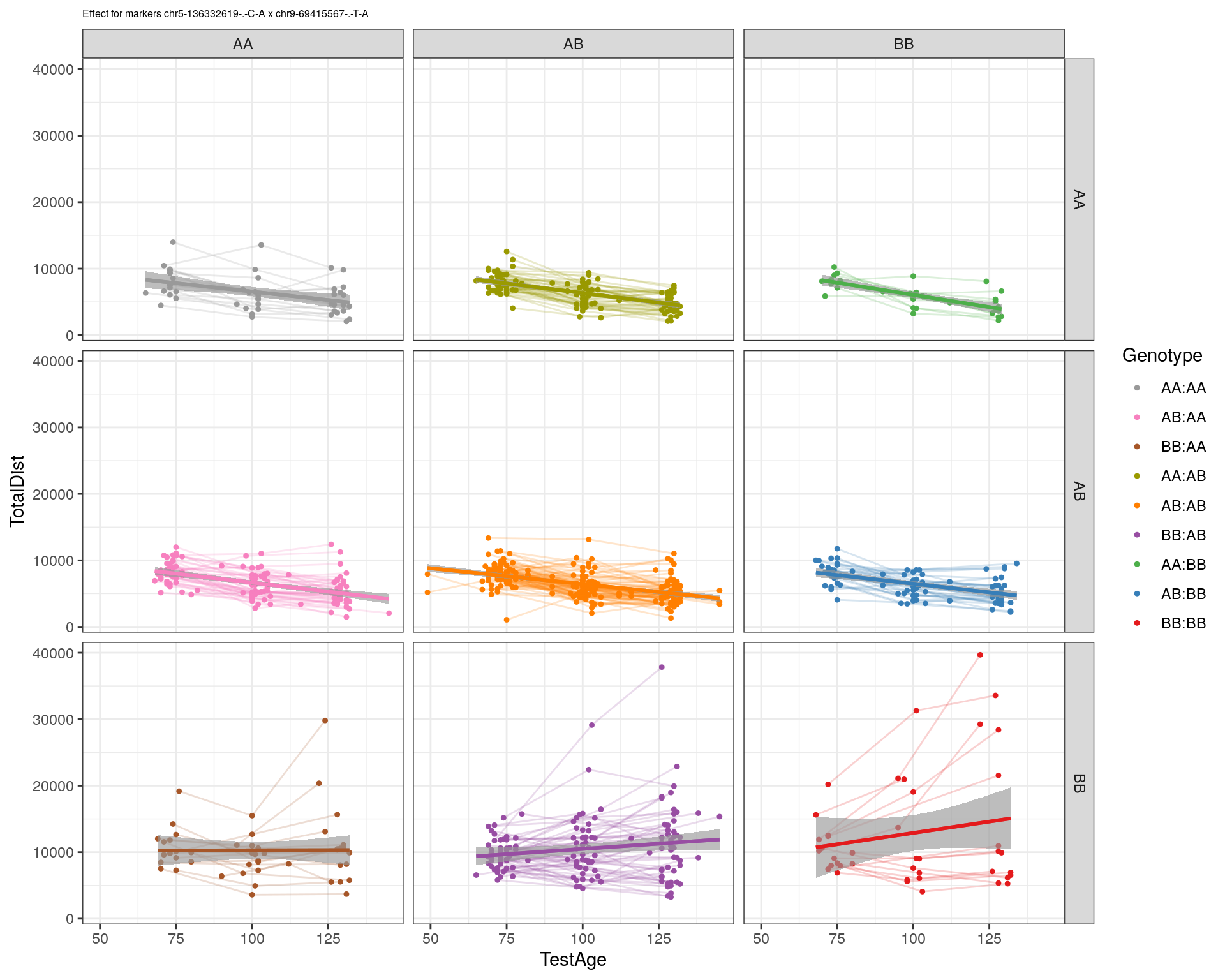
[1] "chr9-71739608-.-T-A"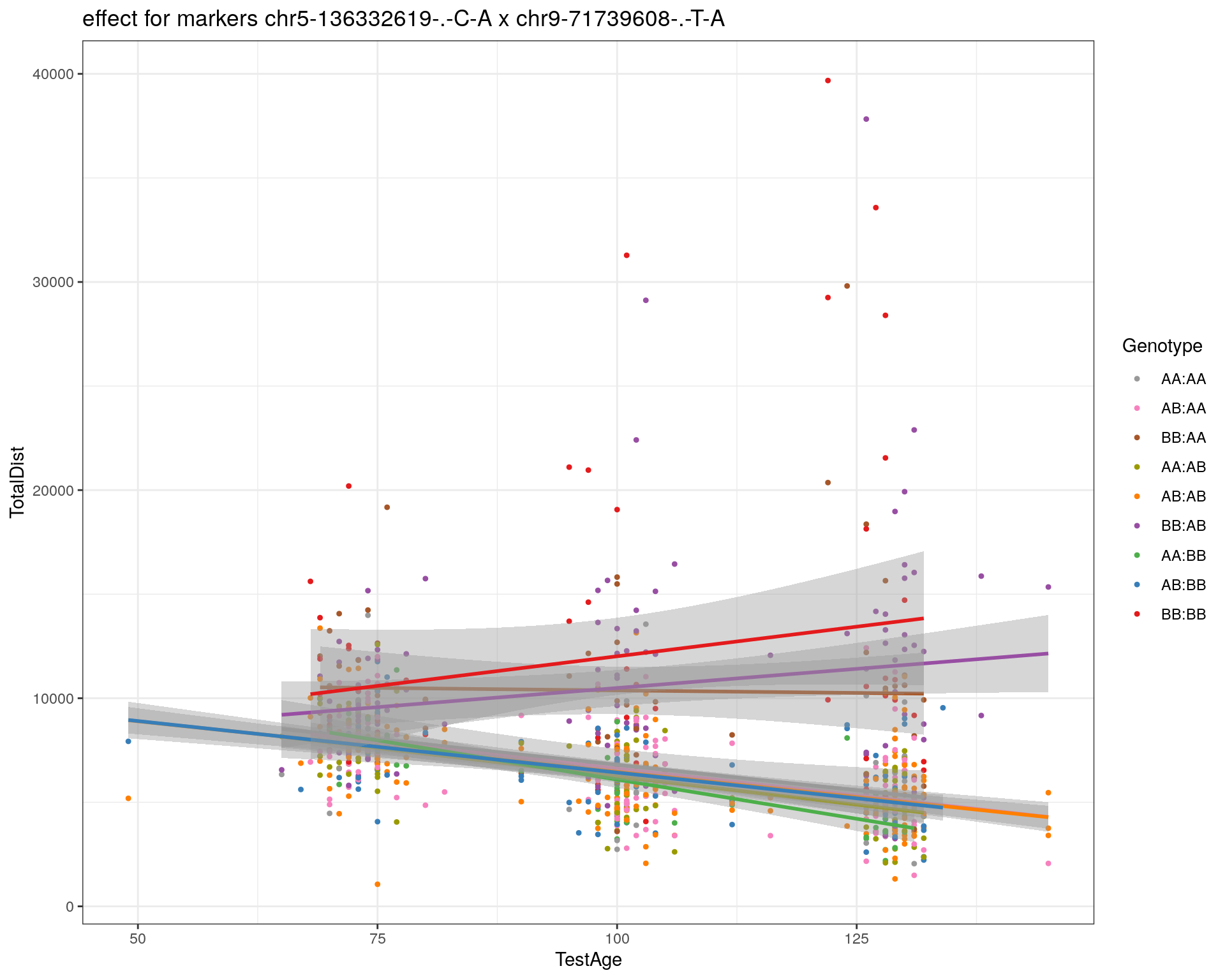

[1] "chr9-80465702-.-T-A"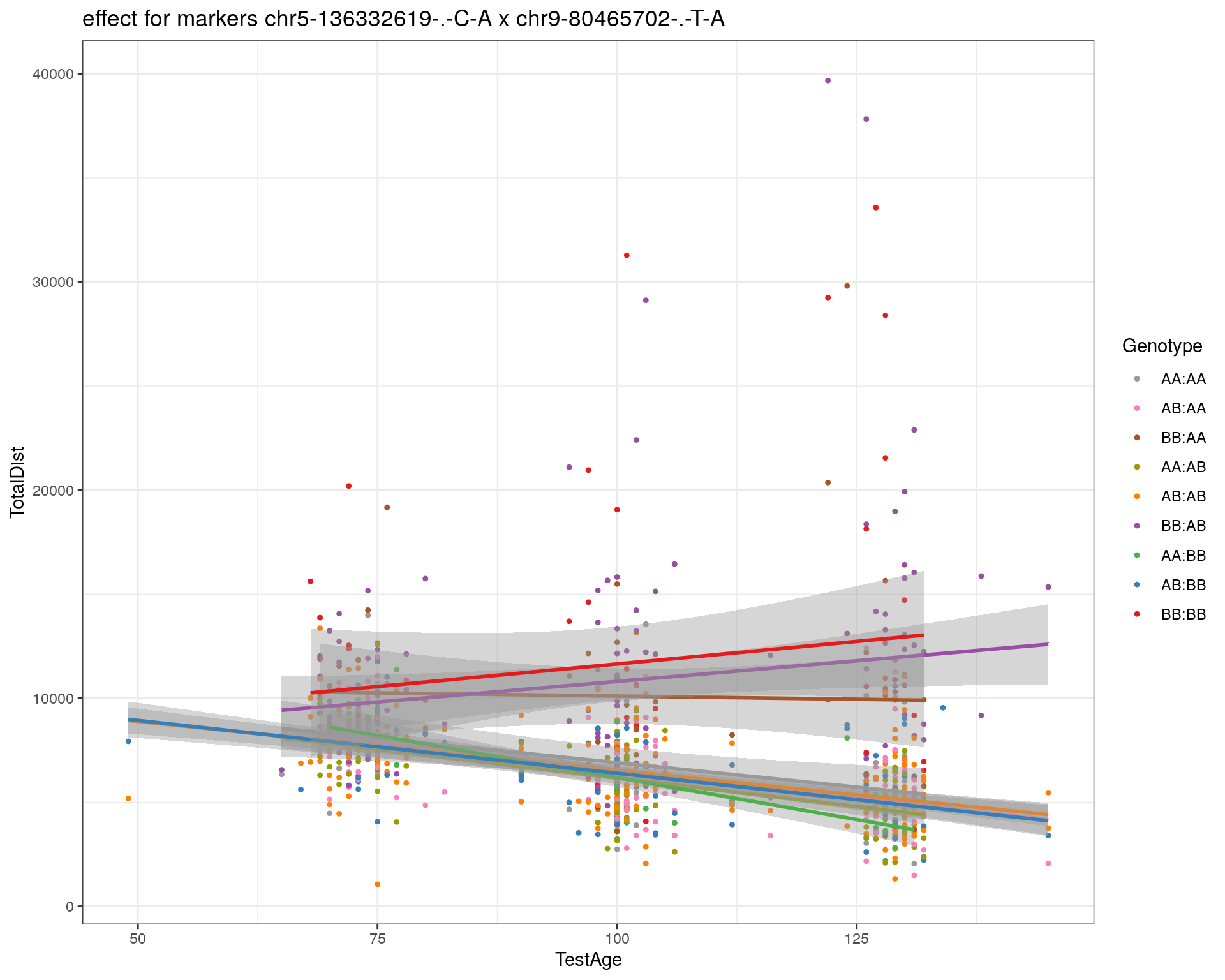
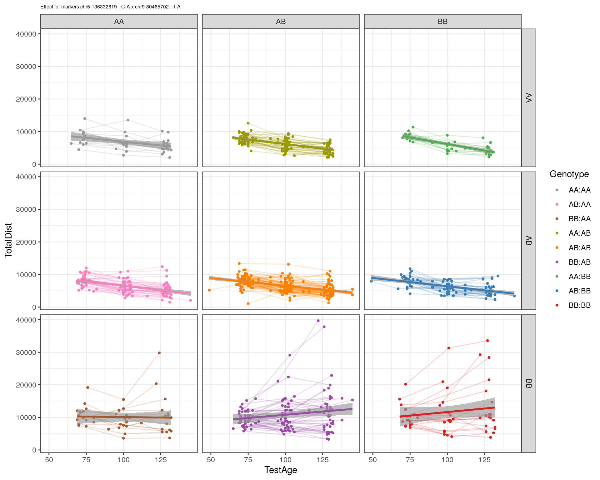
[1] "chr10-24134777-.-A-T"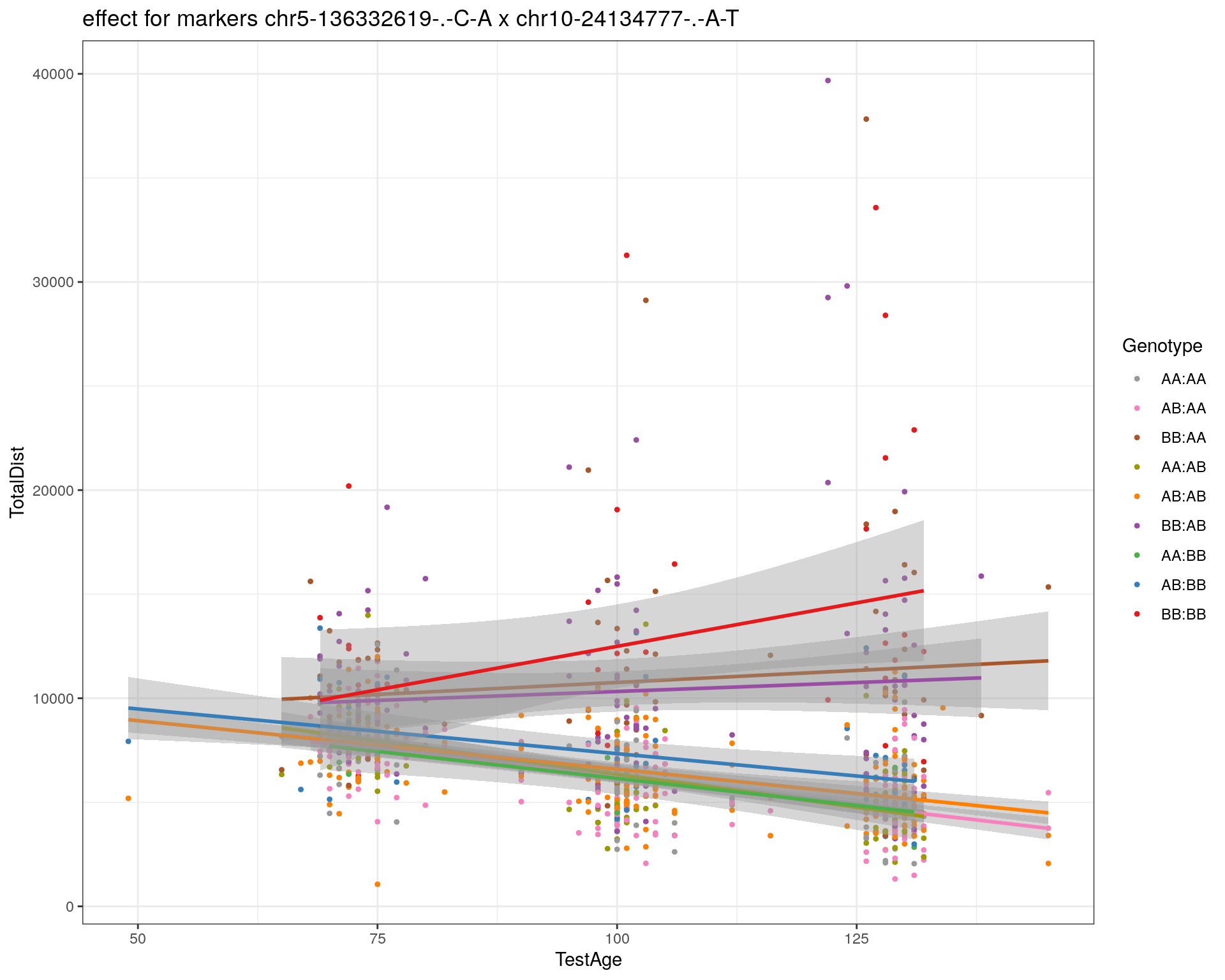
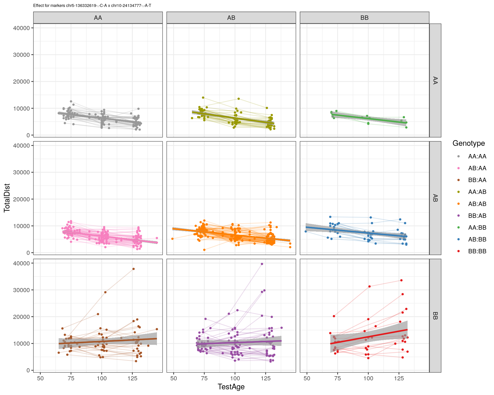
[1] "chr11-96730656-.-A-G"
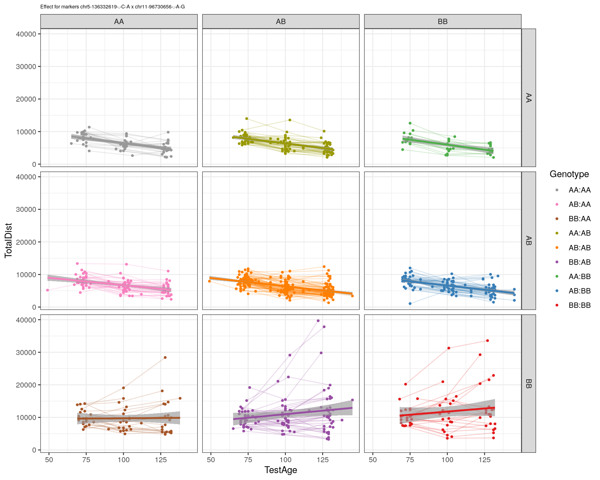
[1] "chr12-43136399-.-A-T"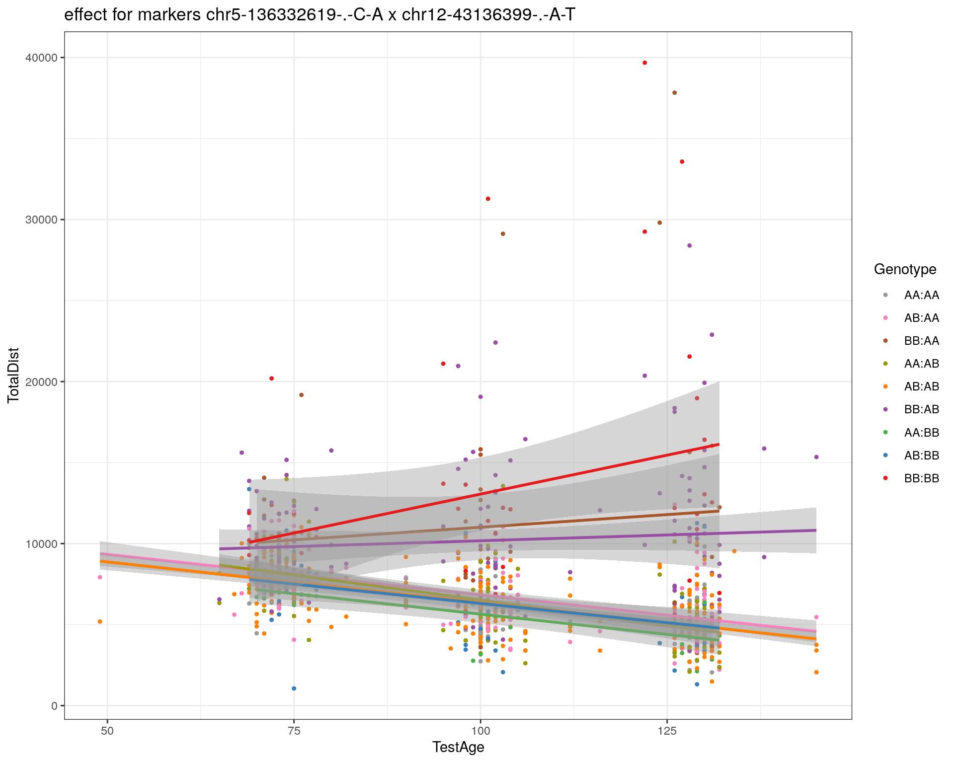
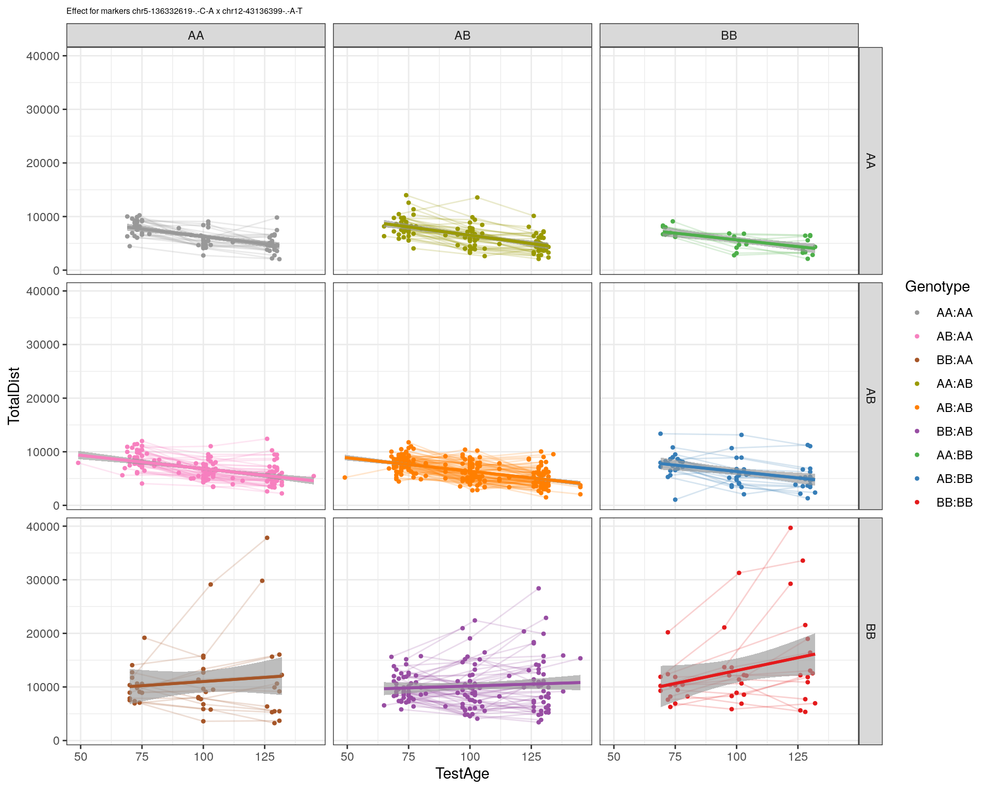
[1] "chr12-69197484-.-C-A"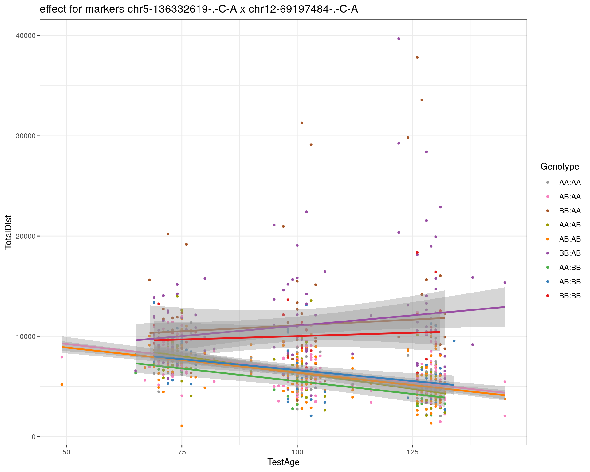
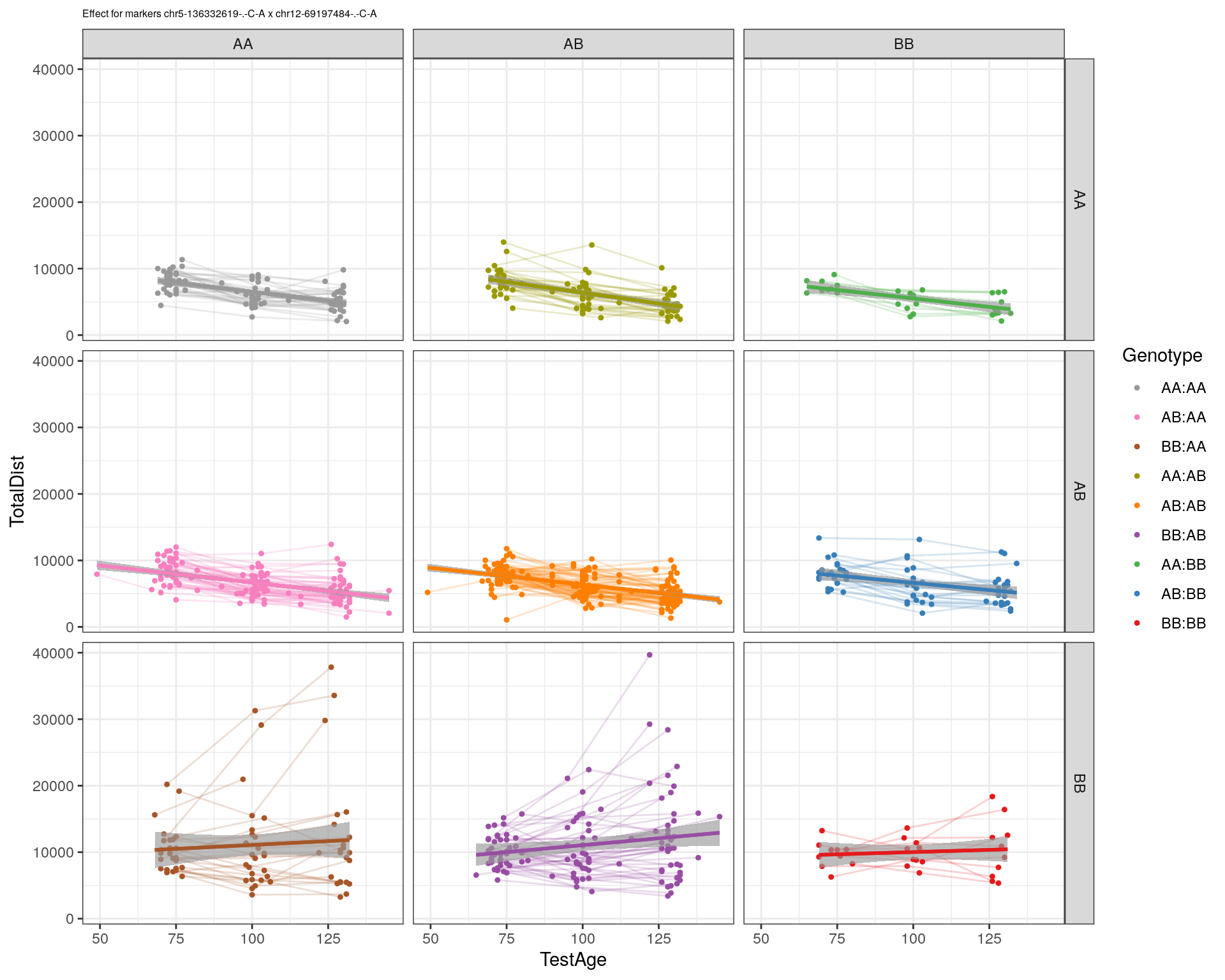
[1] "chr12-86851130-.-T-A"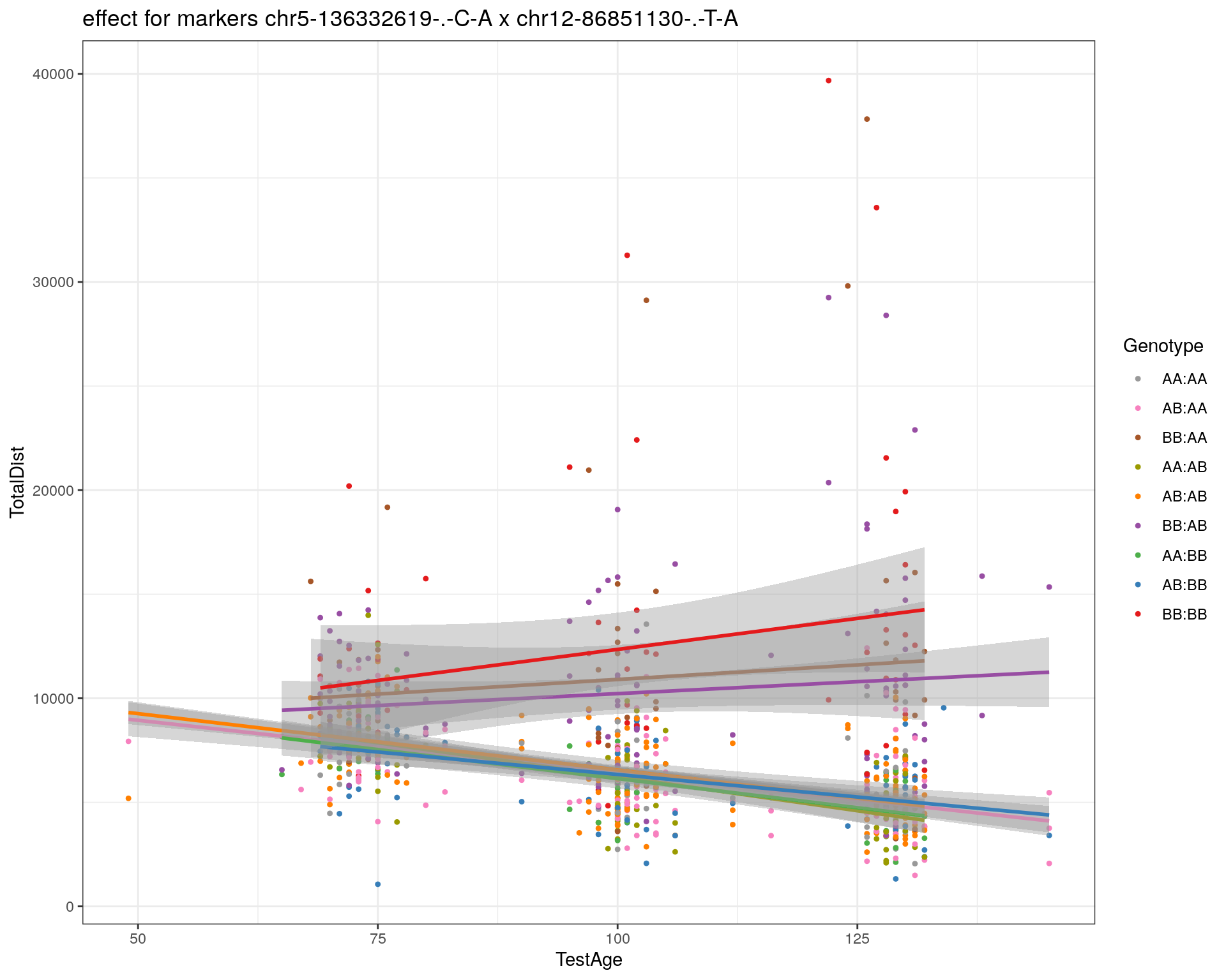
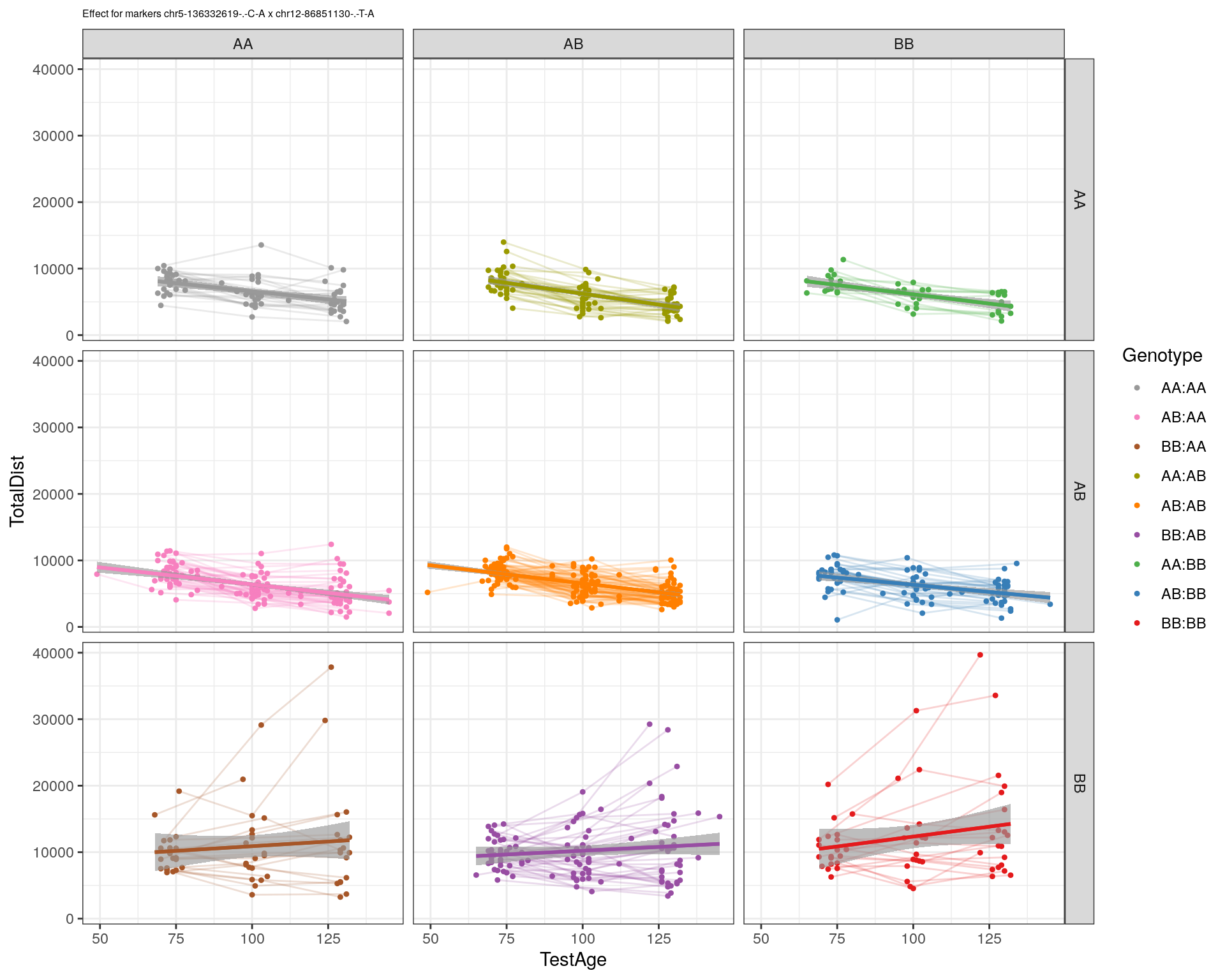
[1] "chr12-112415100-.-G-A"
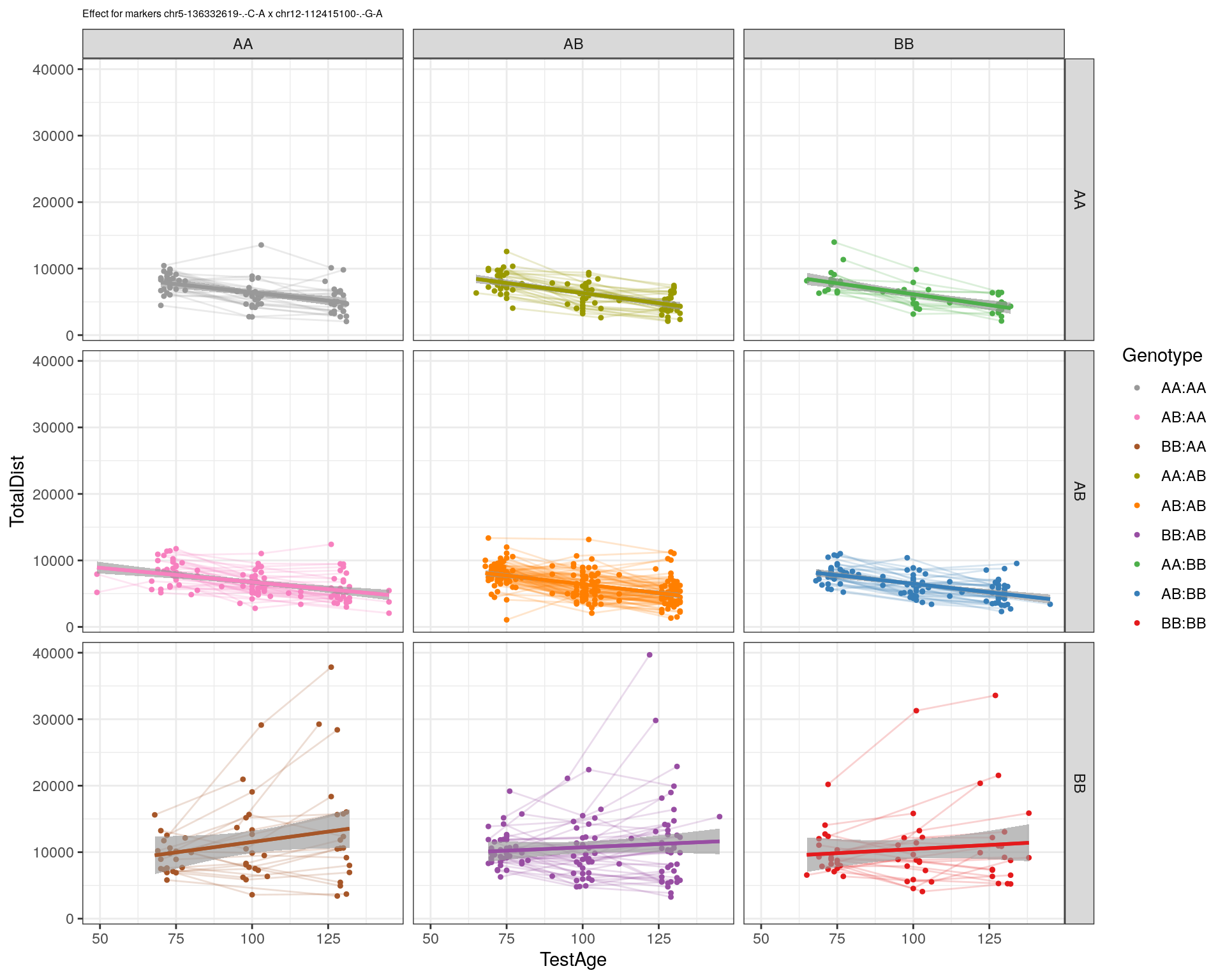
[1] "chr13-20165684-.-T-A"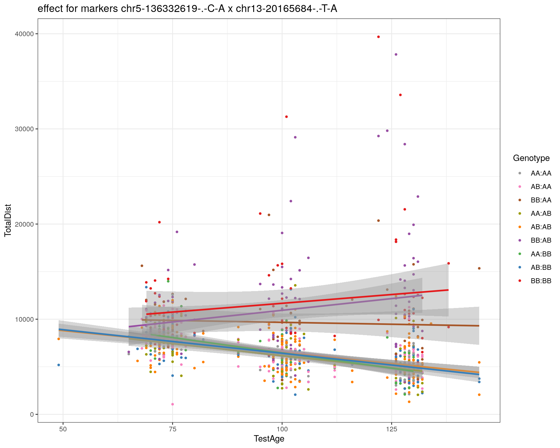

[1] "chr13-115031098-.-T-C"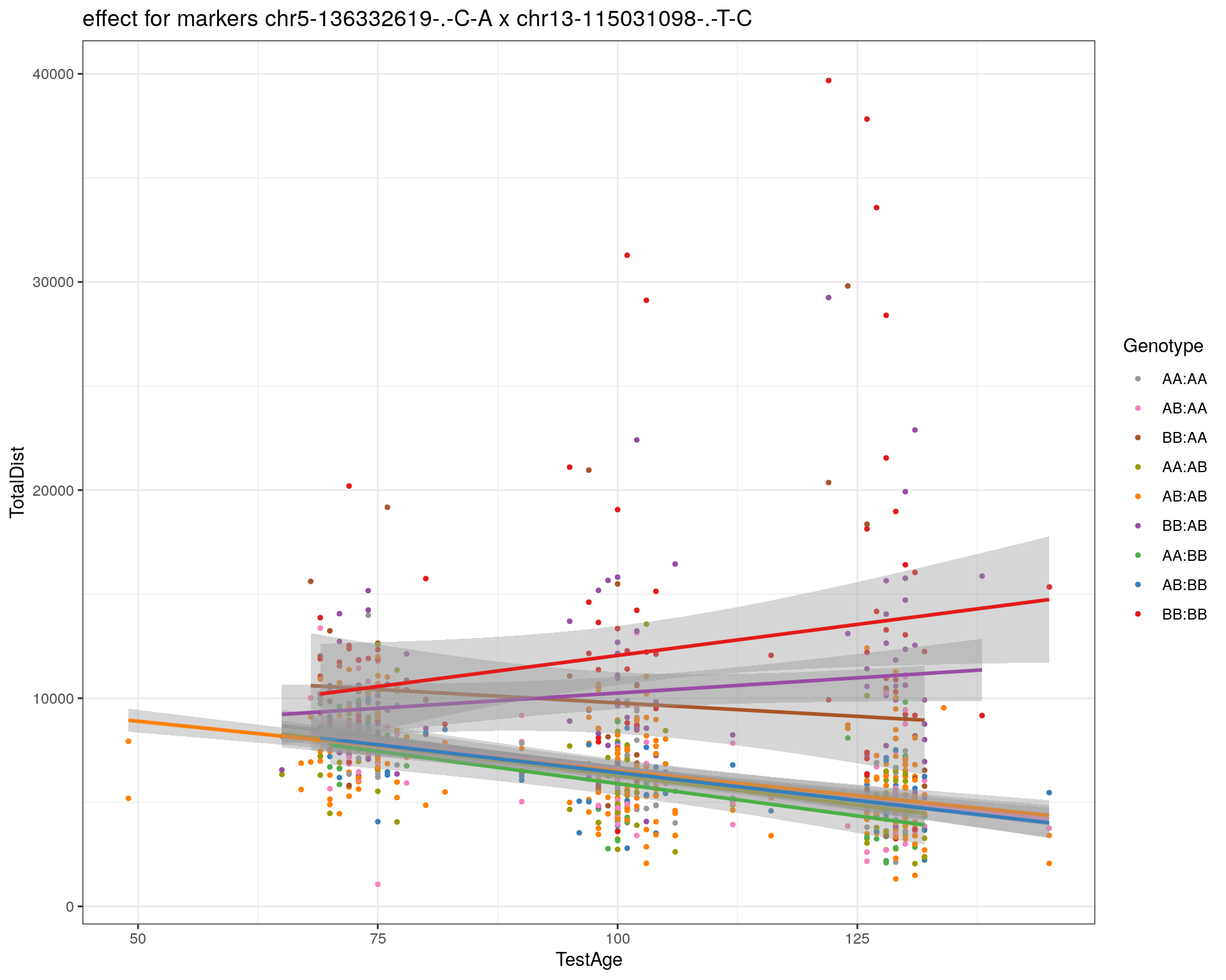

[1] "chr14-11709591-.-T-C"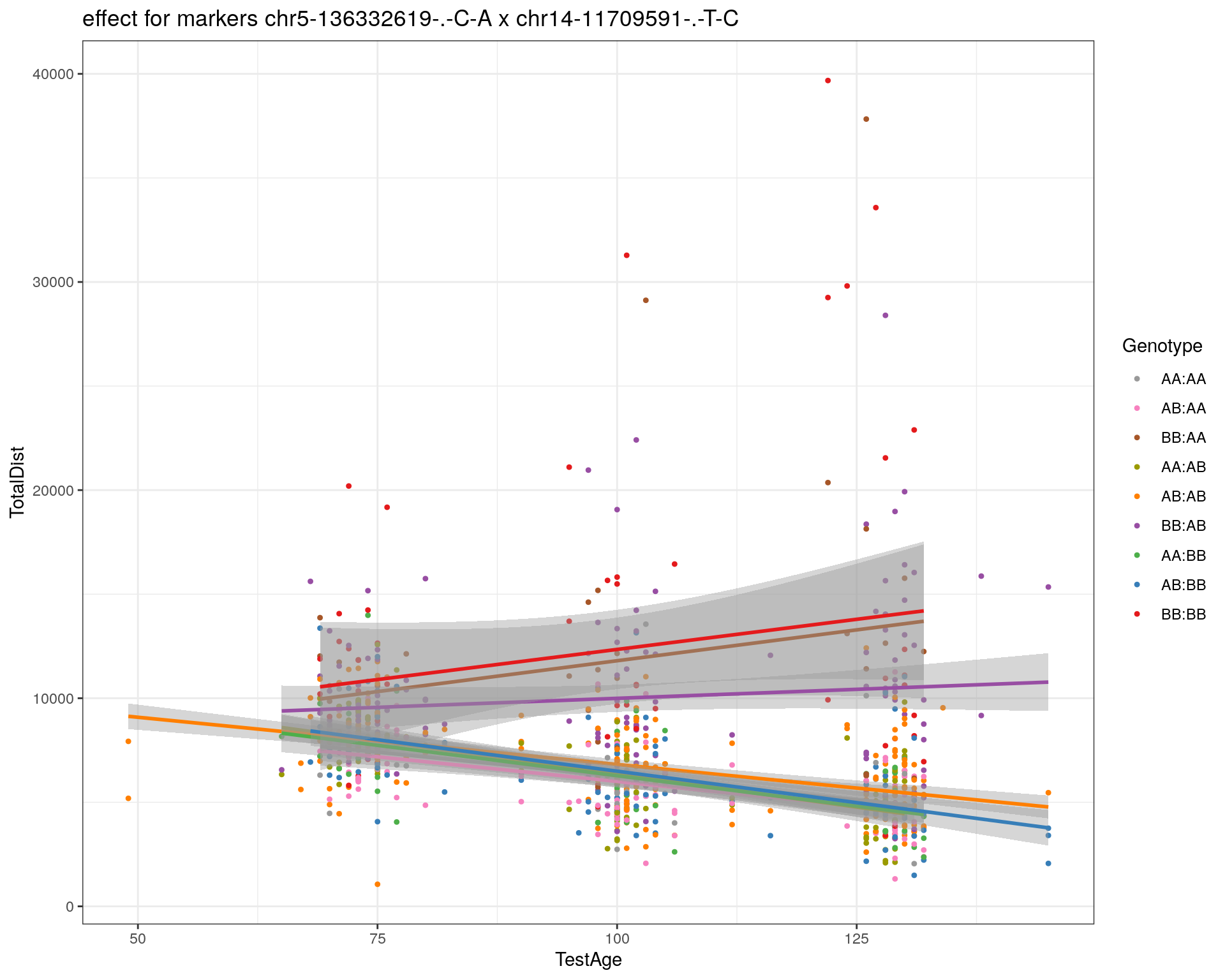

[1] "chr14-50642778-.-G-A"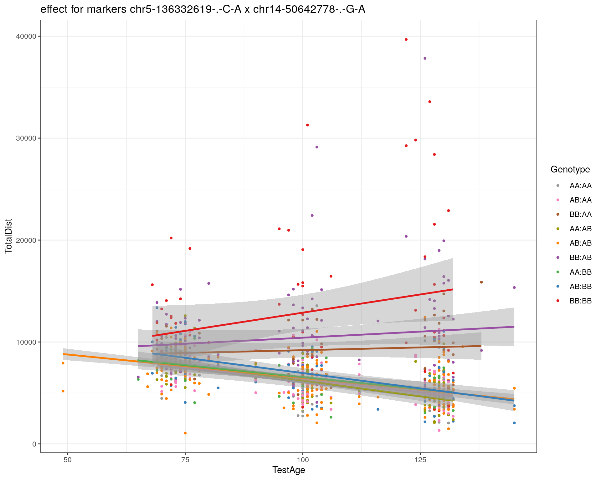
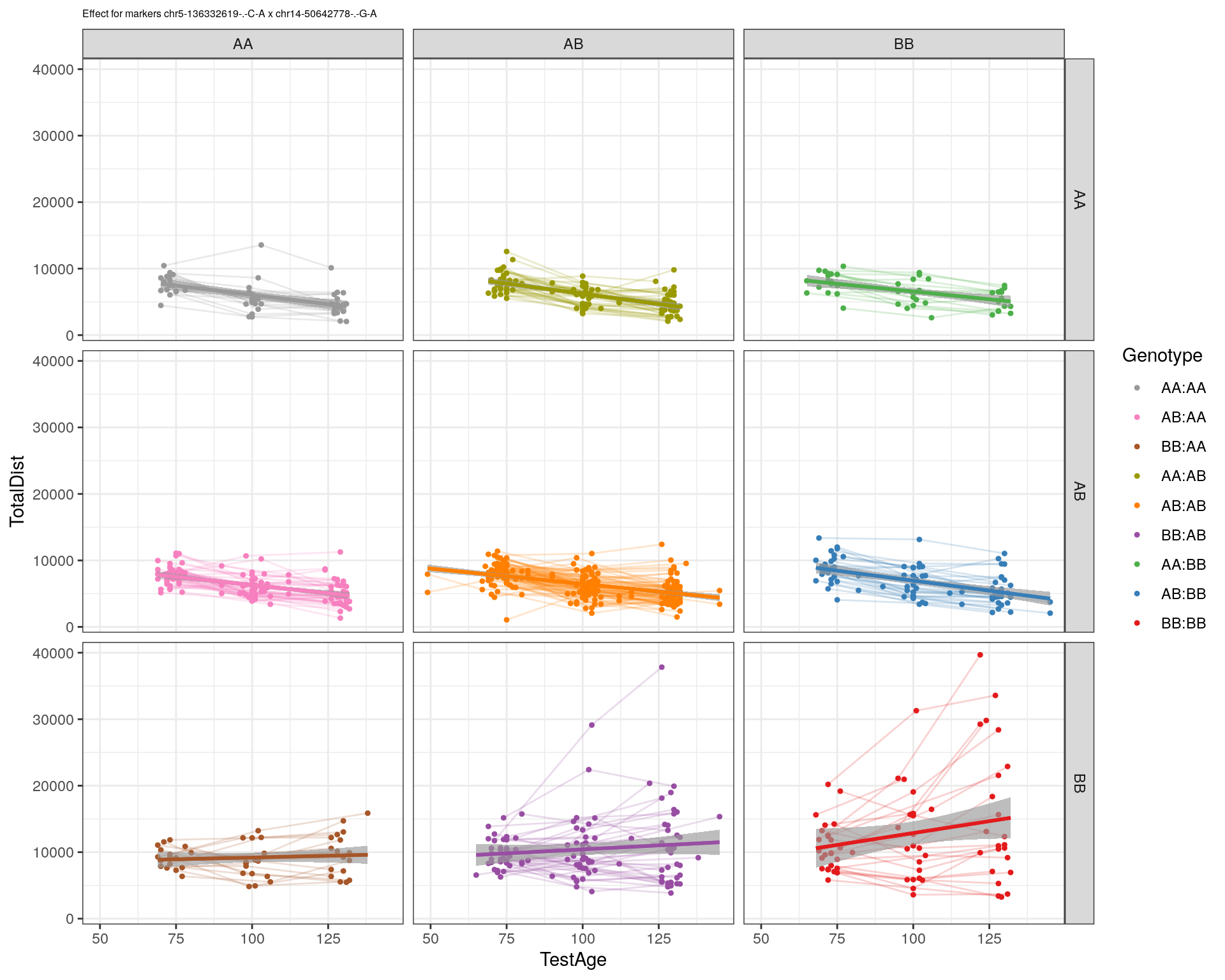
[1] "chr14-62407765-.-T-A"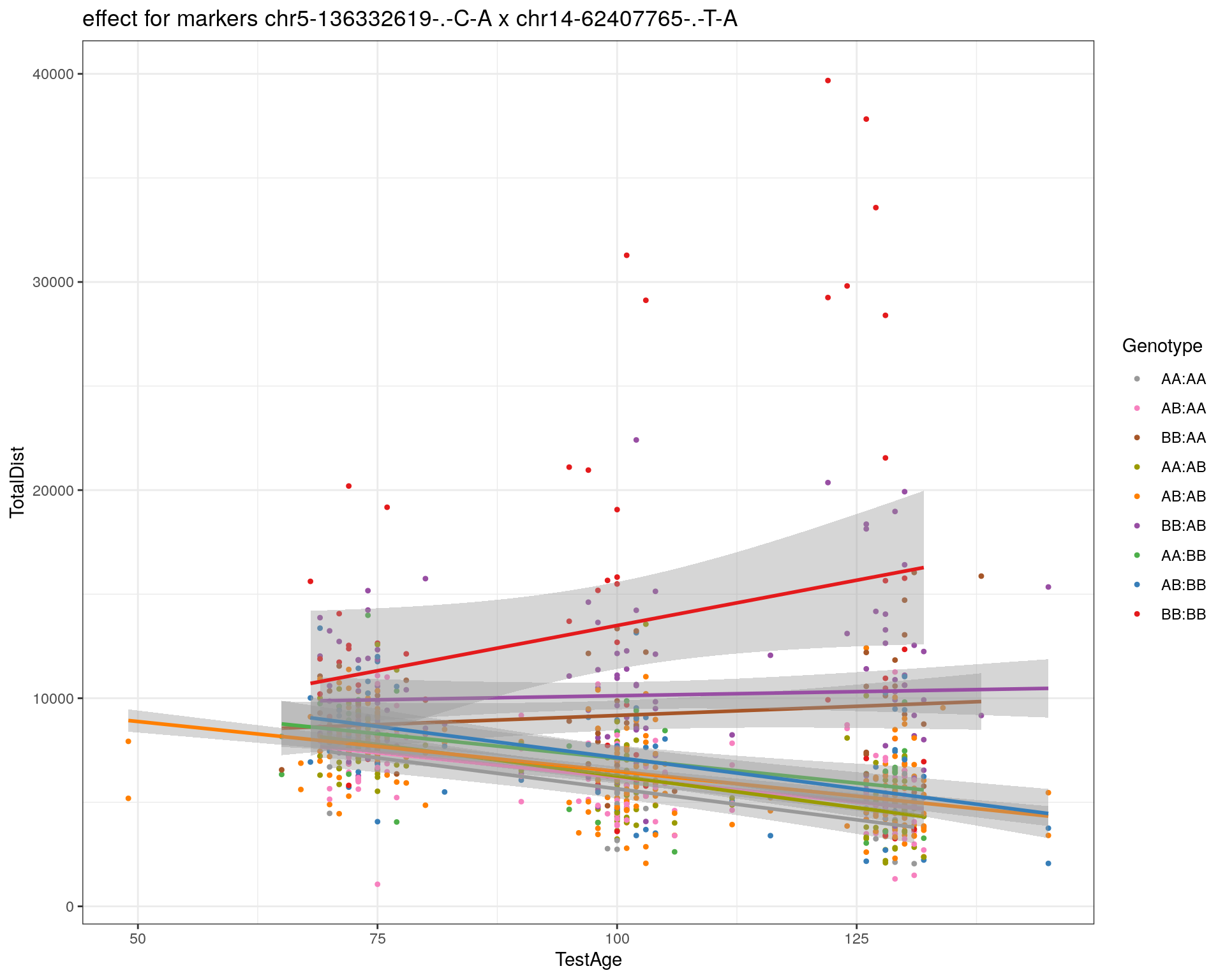
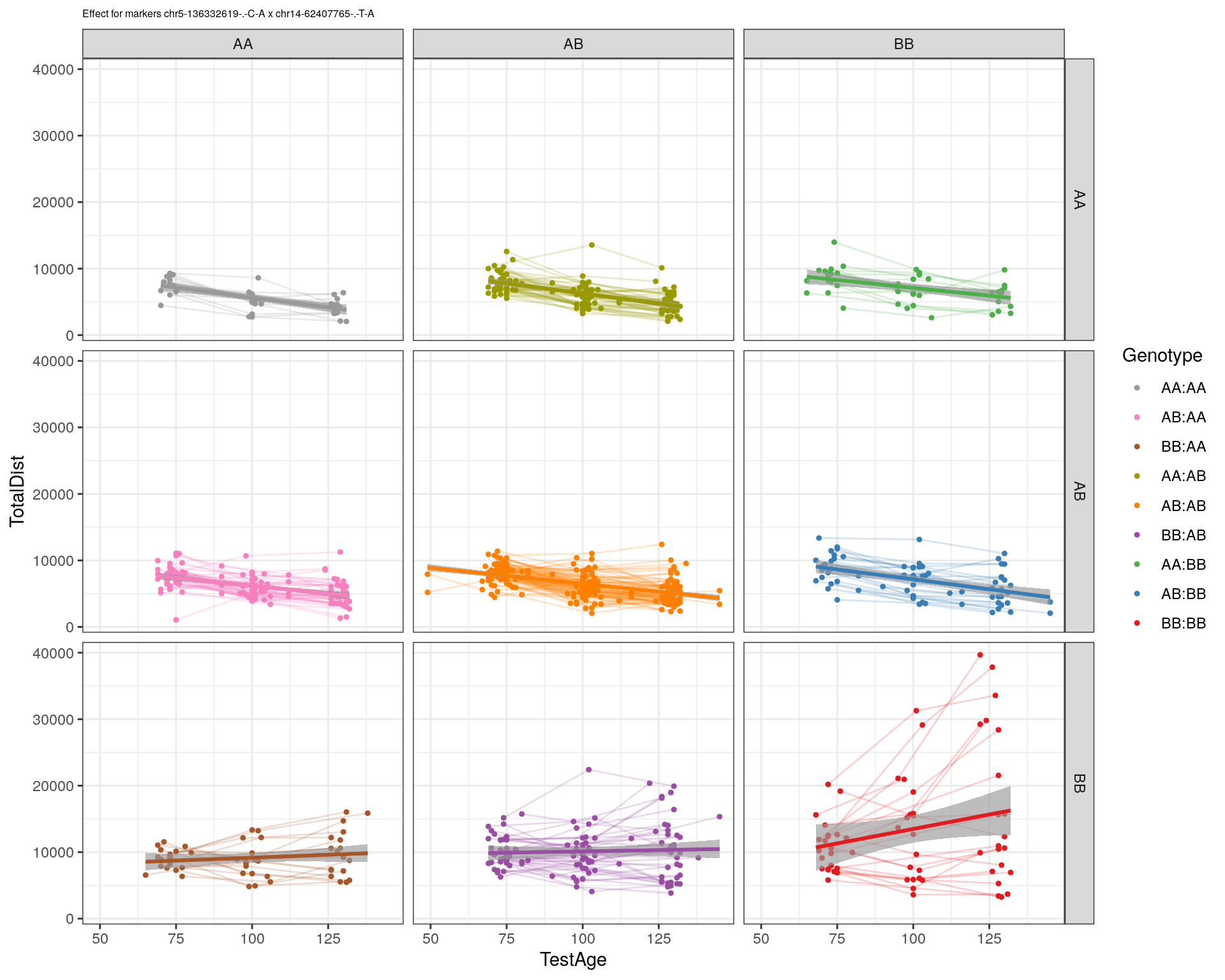
[1] "chr14-69691477-.-G-T"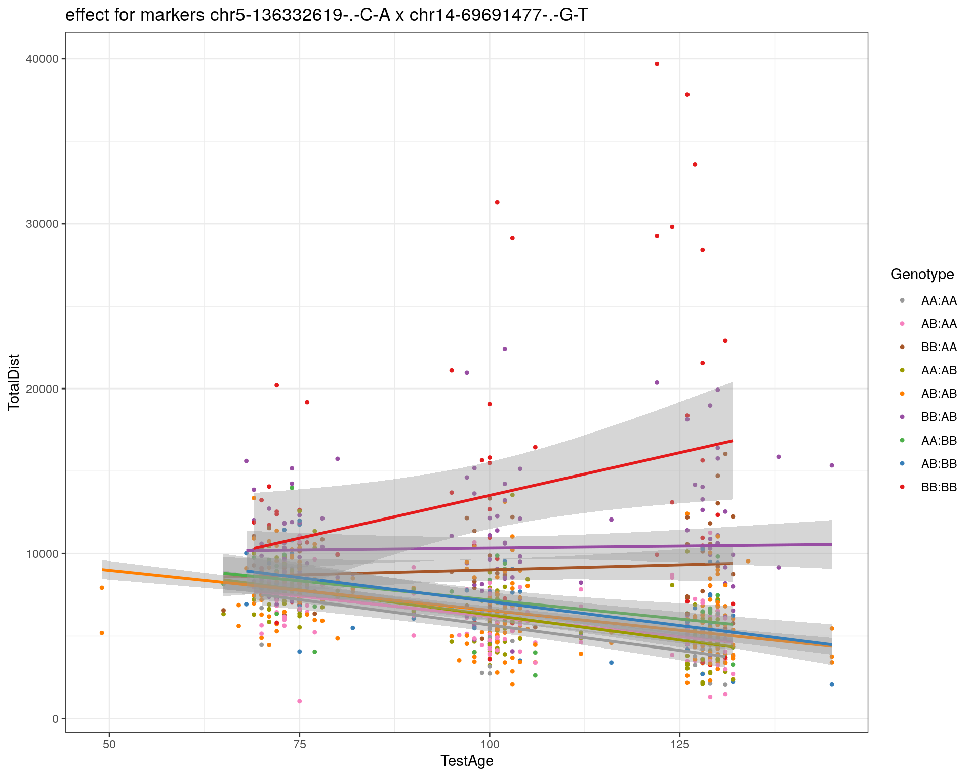
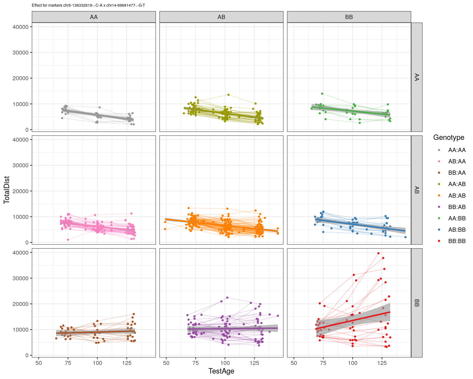
[1] "chr15-58605950-.-C-G"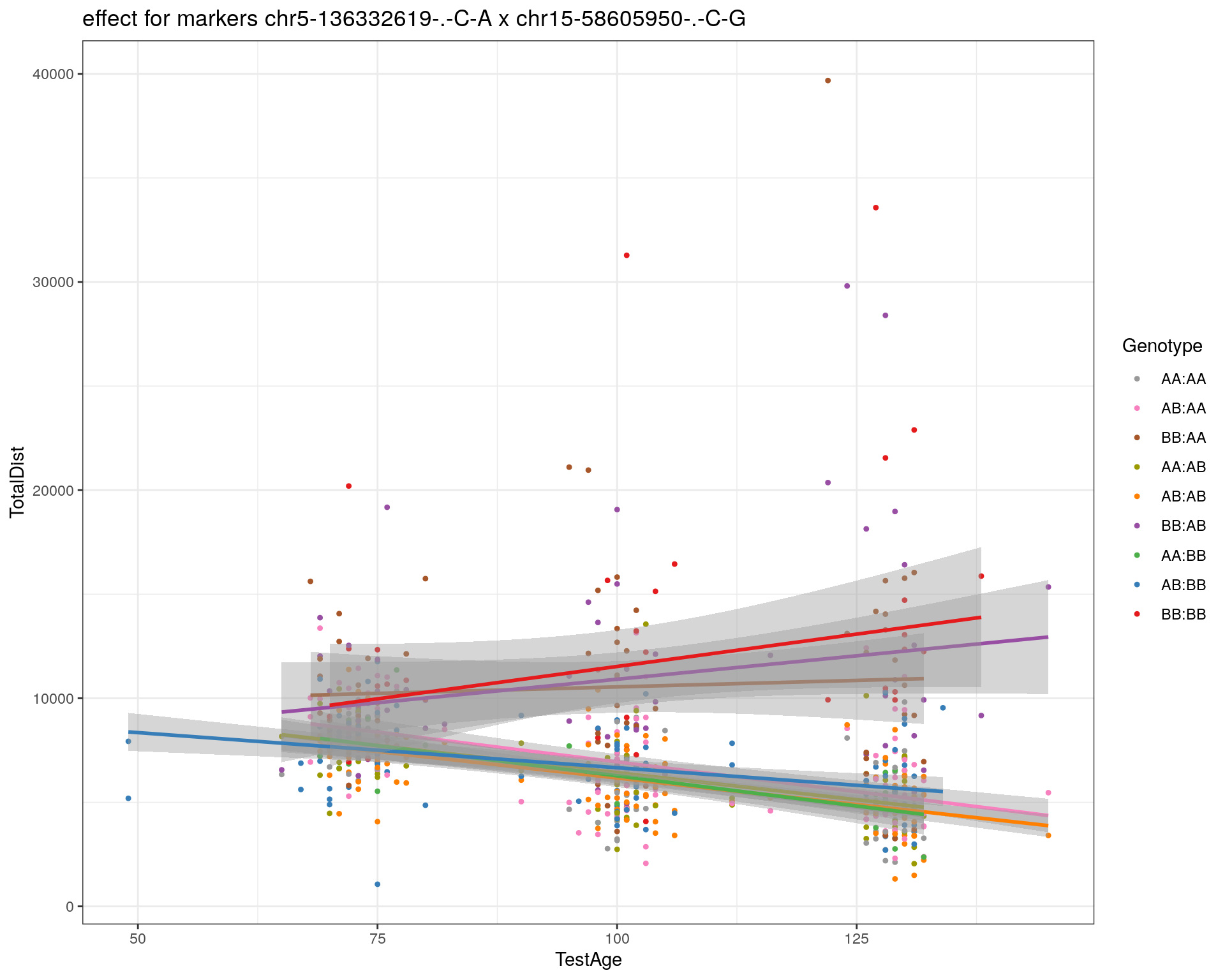
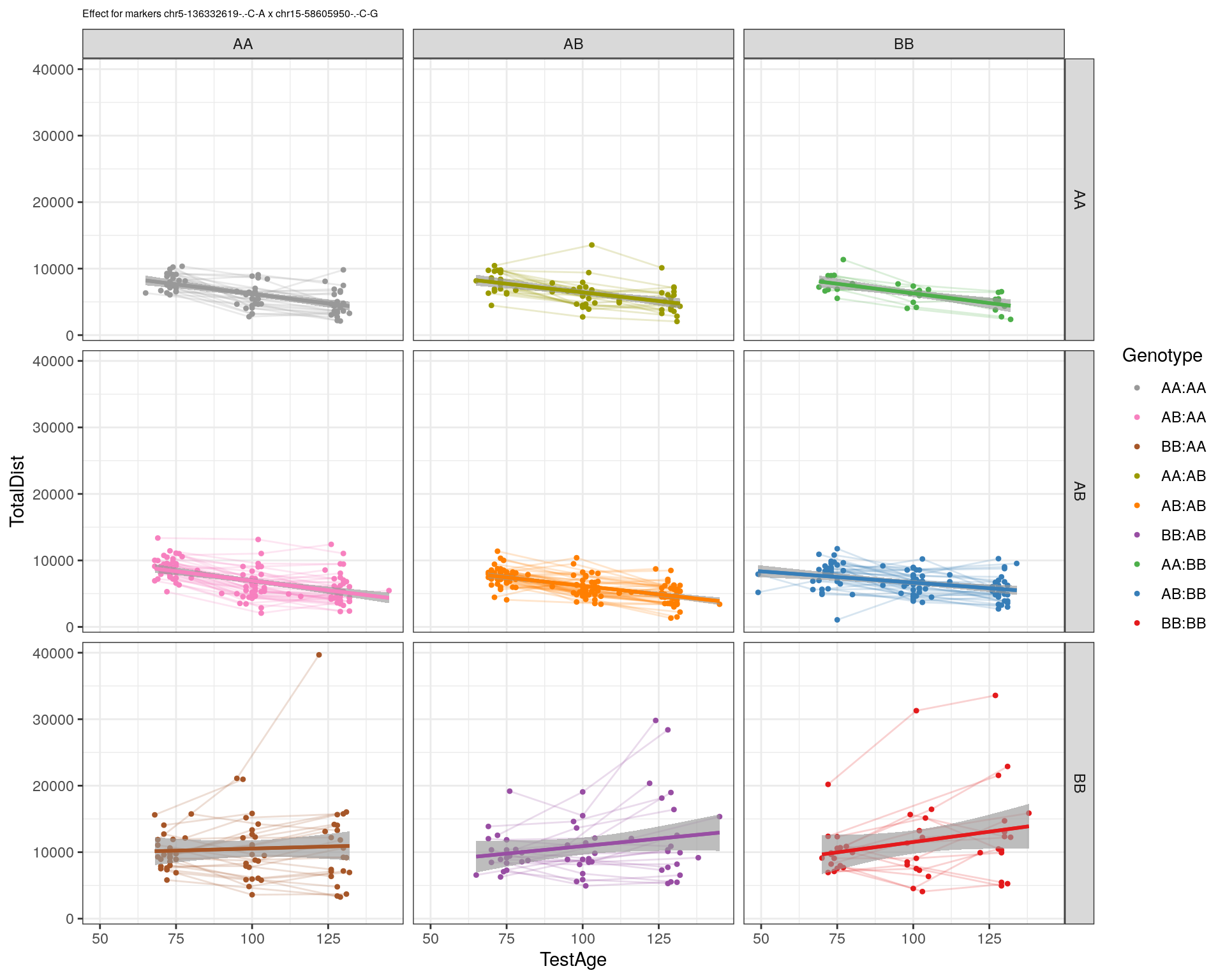
[1] "chr15-74727869-.-C-T"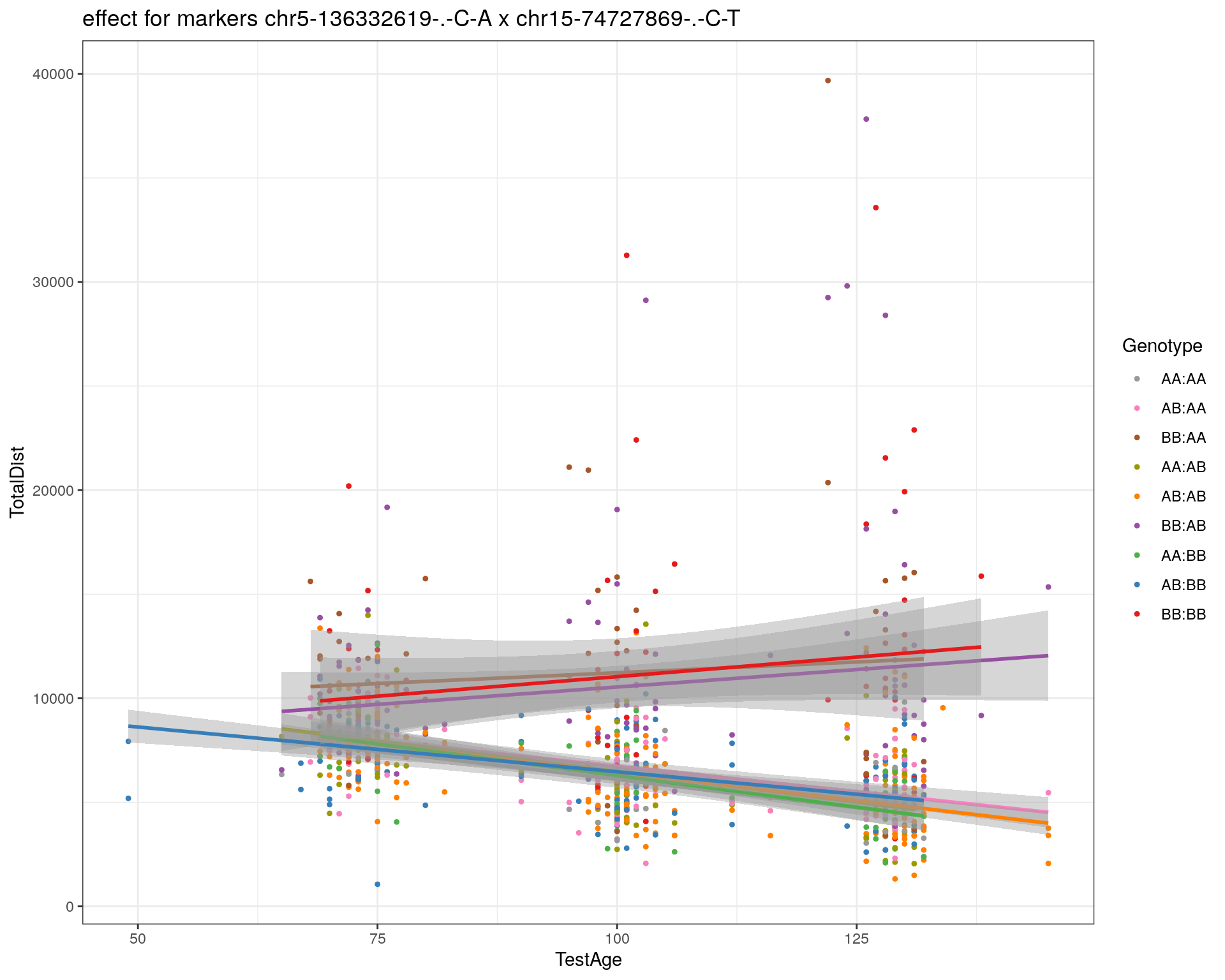
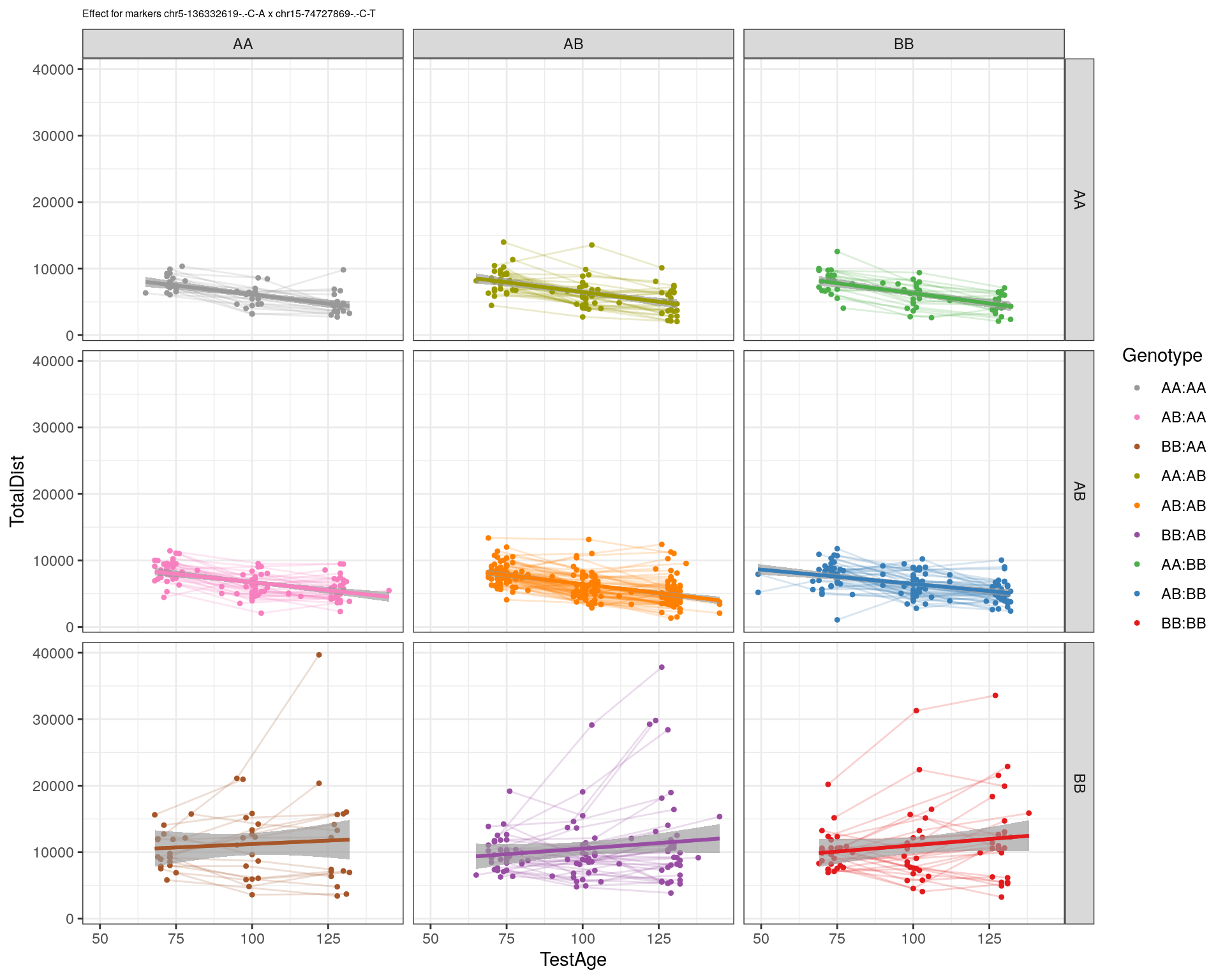
[1] "chr16-32593683-.-A-G"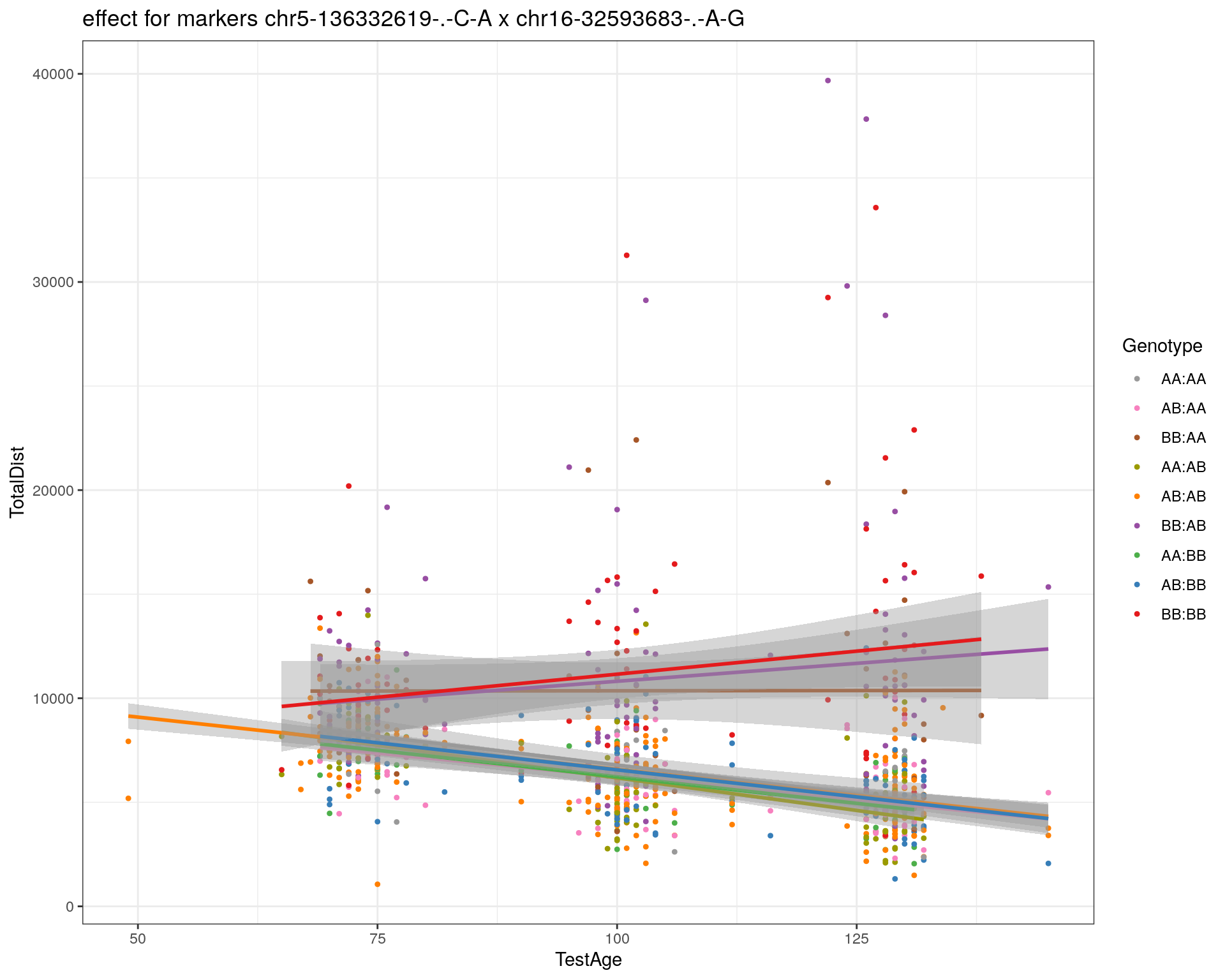

[1] "chr16-75648687-.-G-A"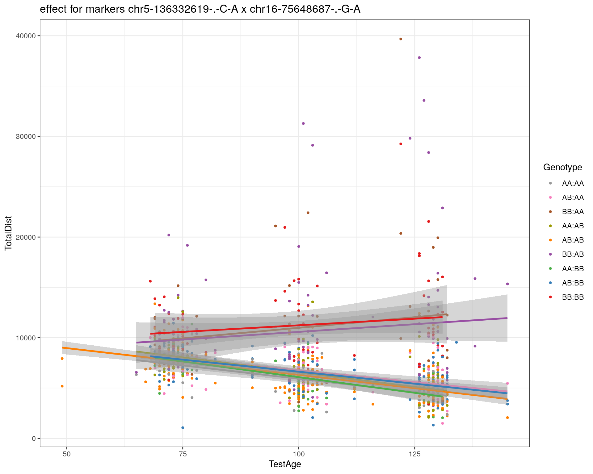
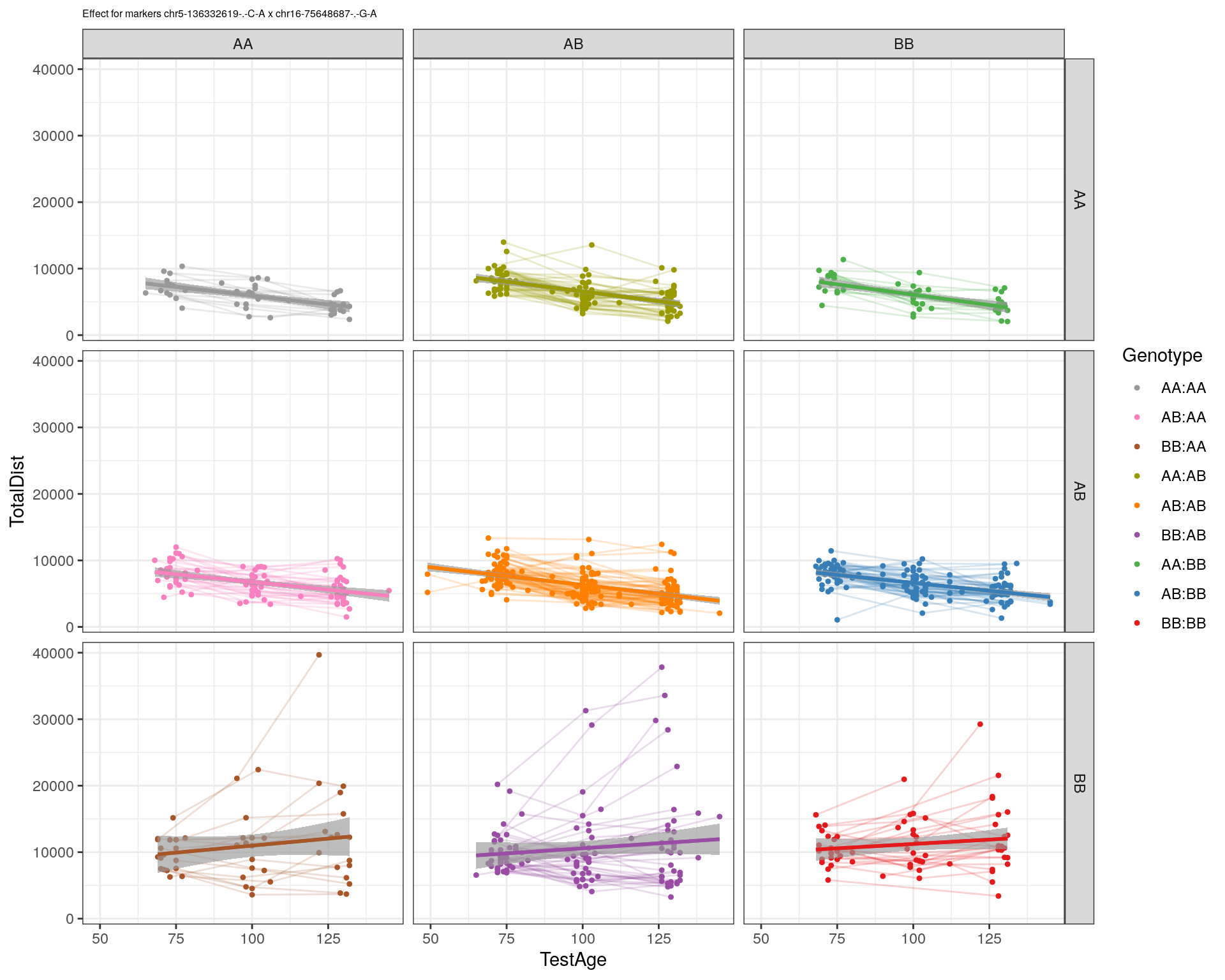
[1] "chr17-61305603-.-G-A"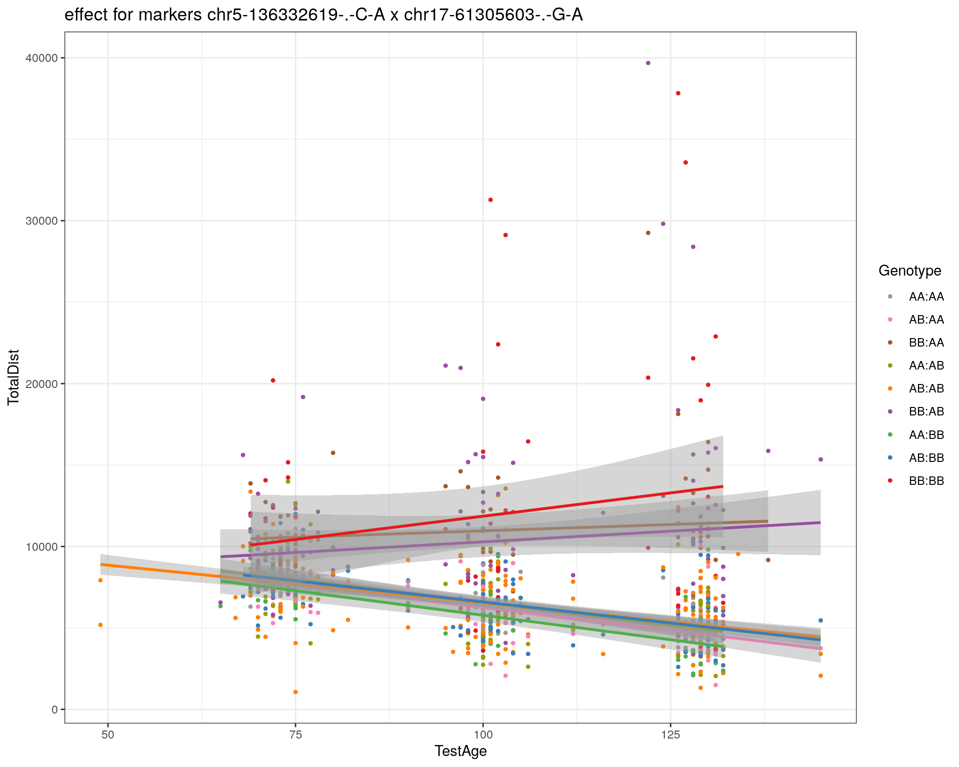
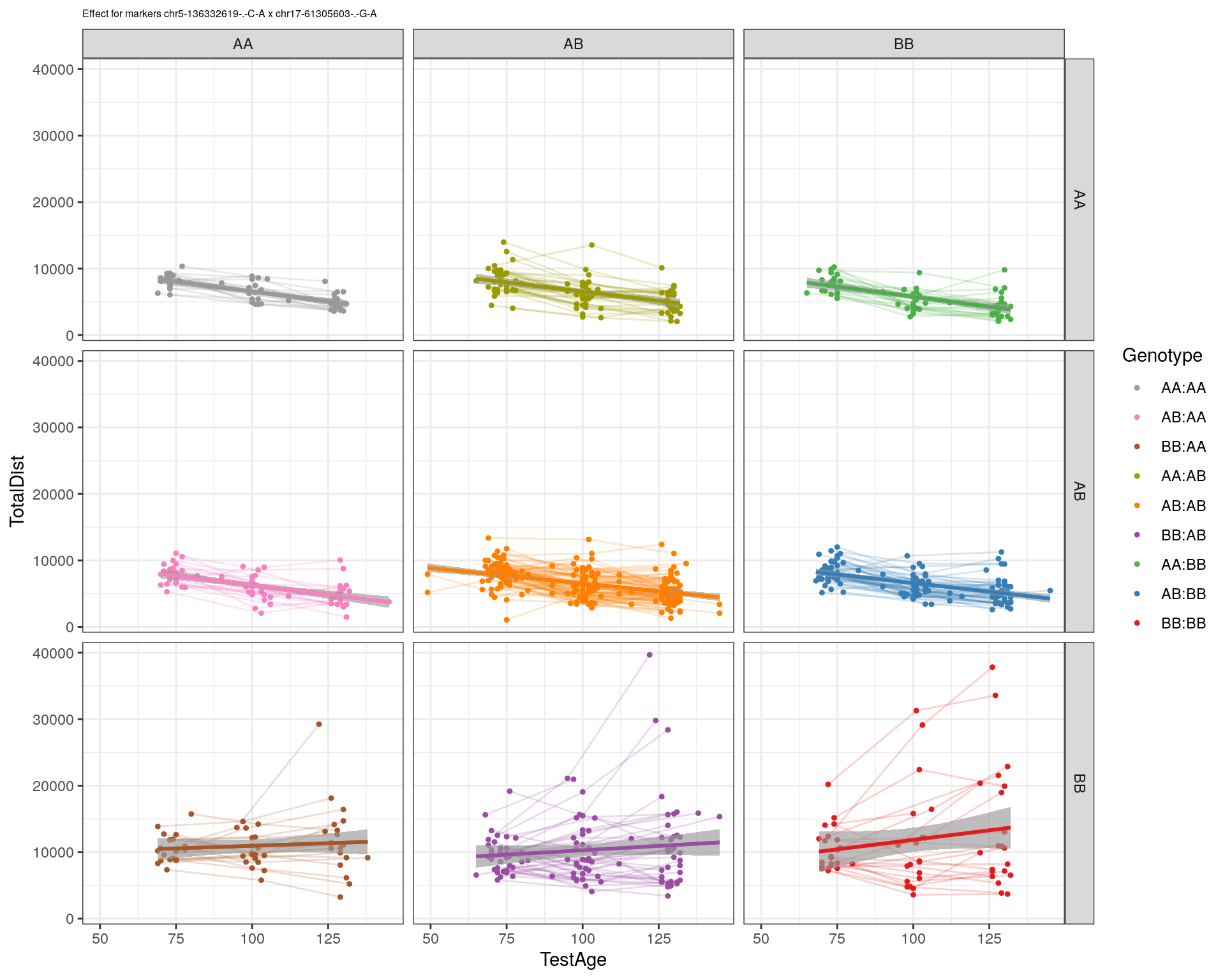
[1] "chr17-69219676-.-G-A"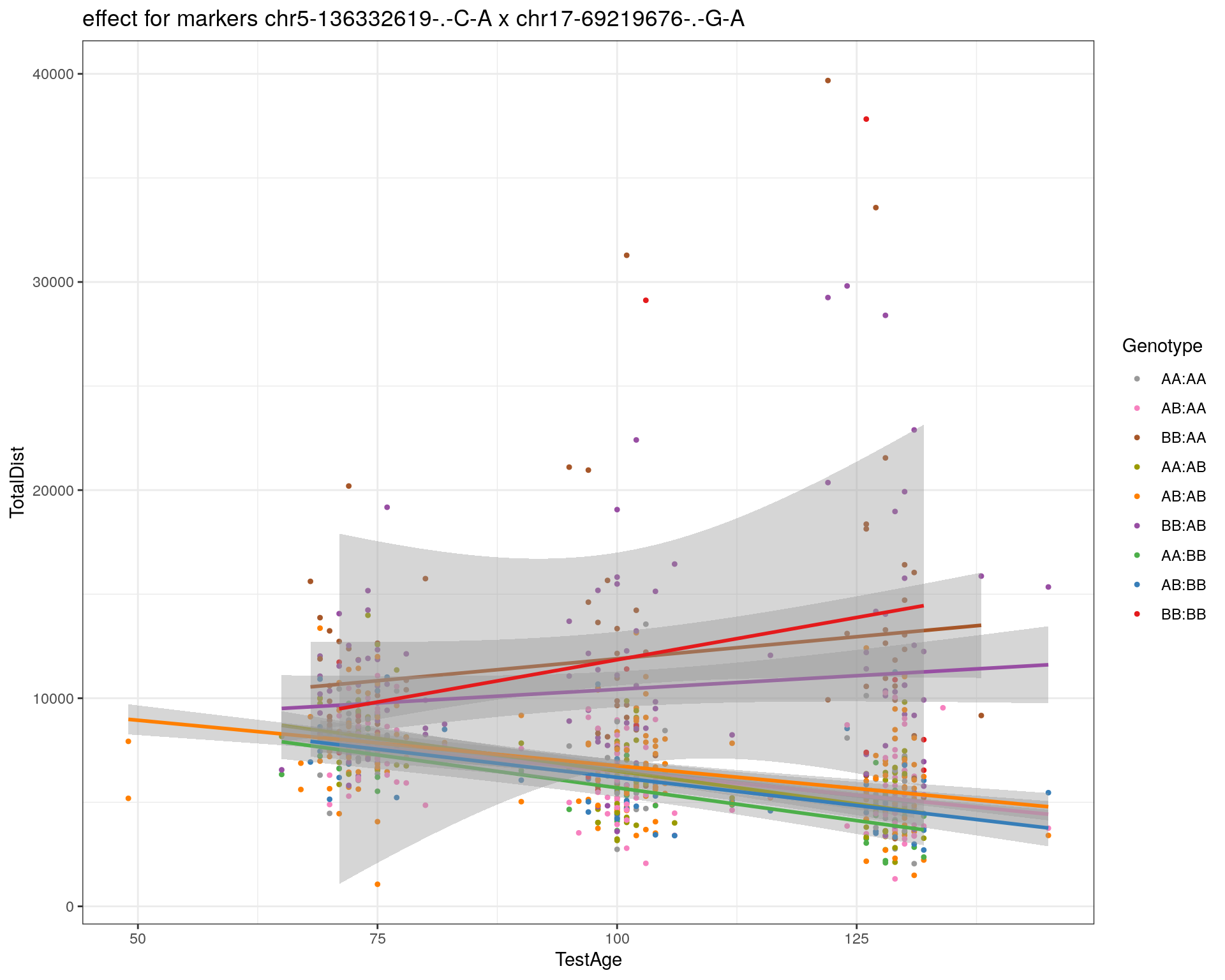
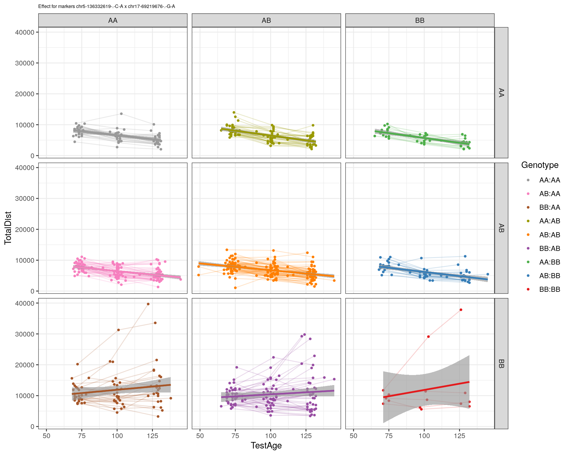
[1] "chr18-51300216-.-T-A"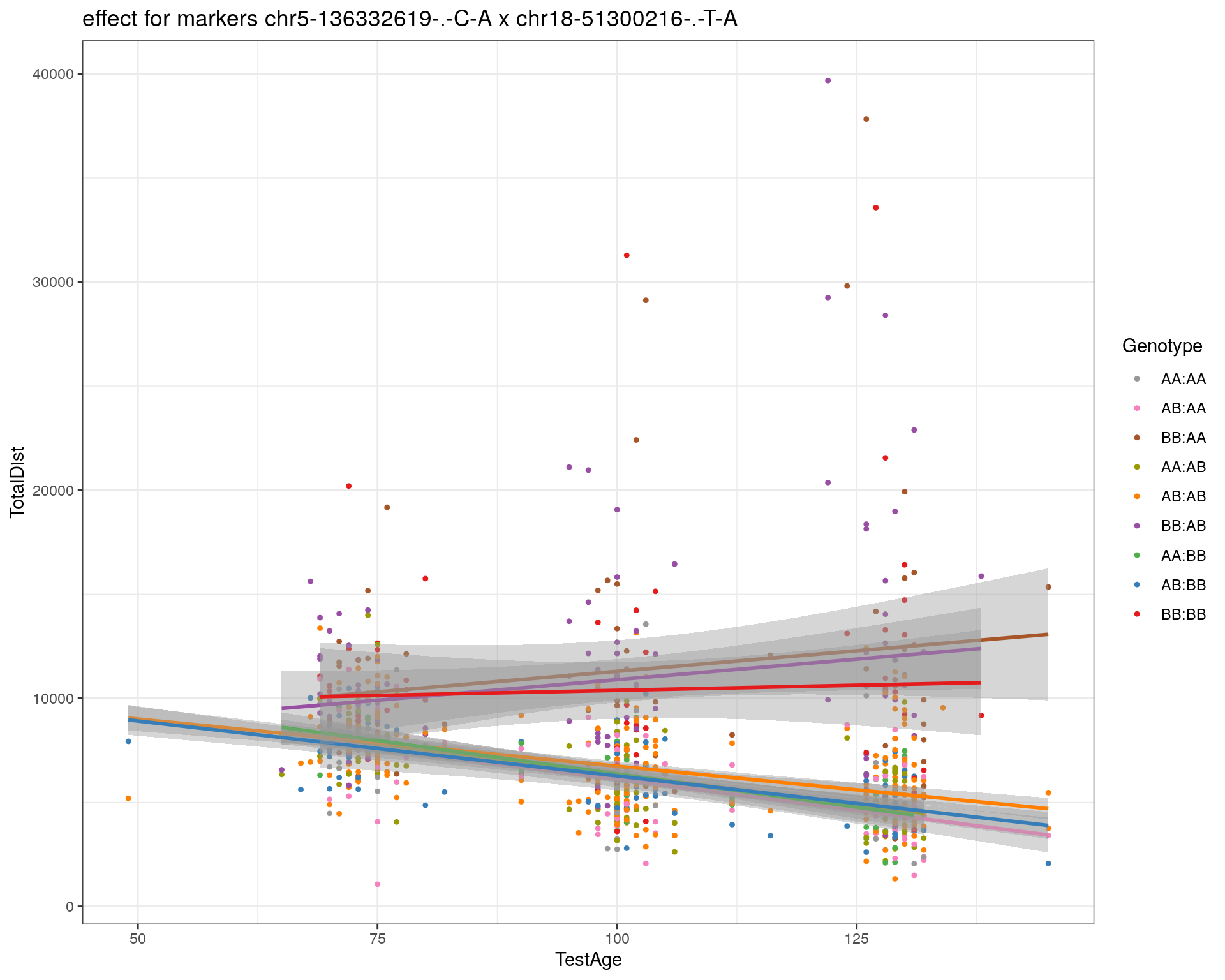
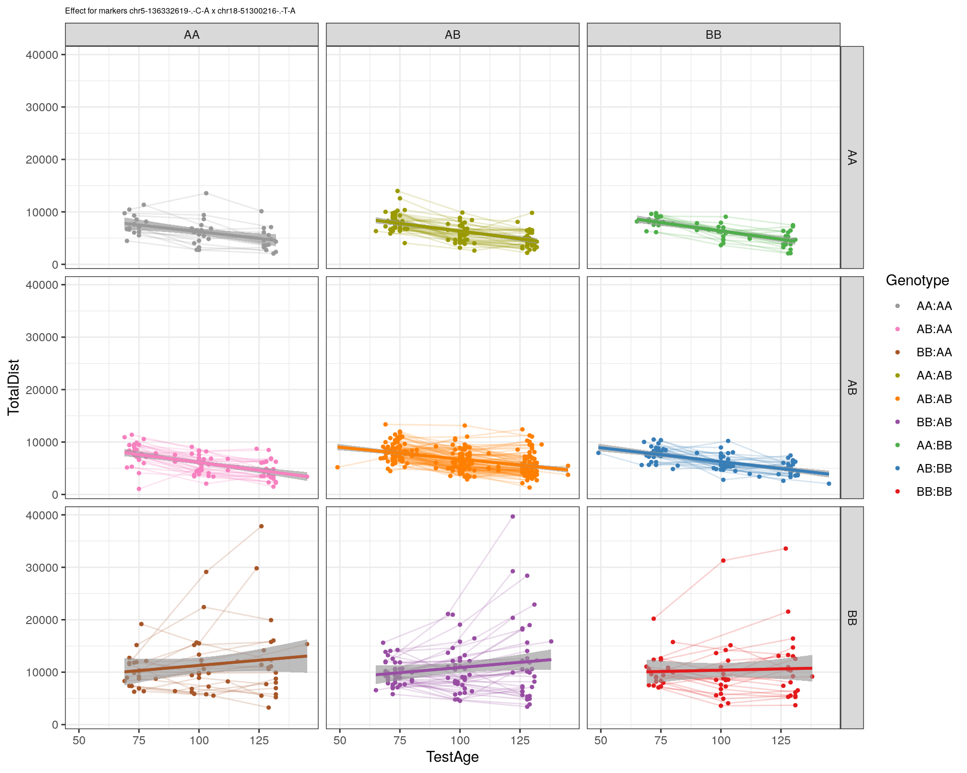
[1] "chr18-89347666-.-A-G"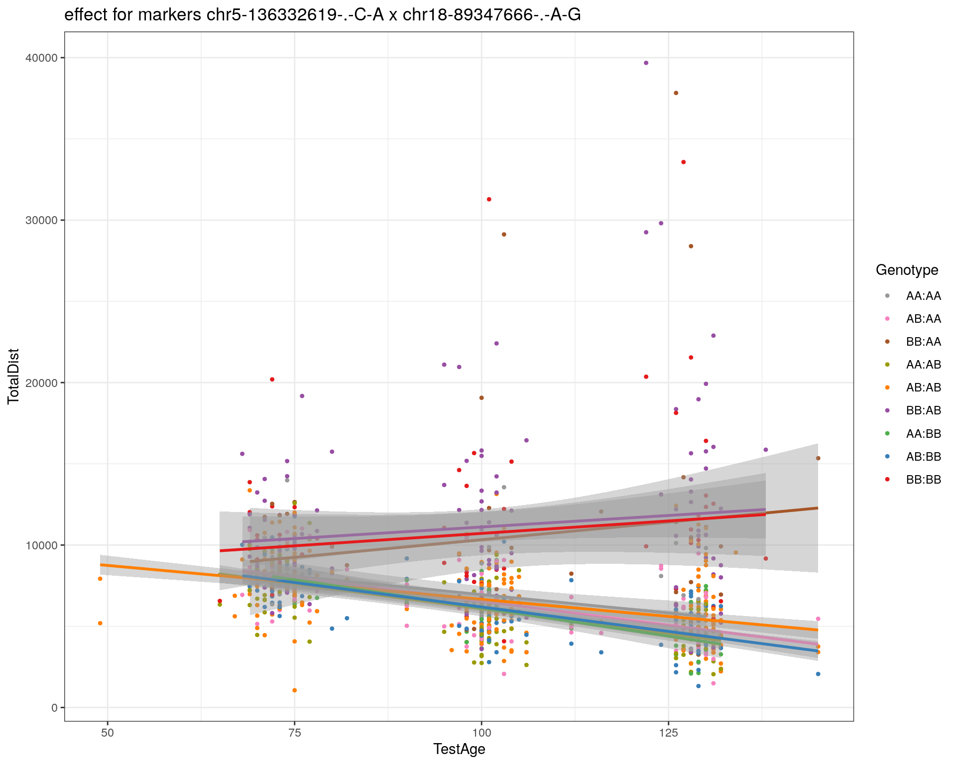
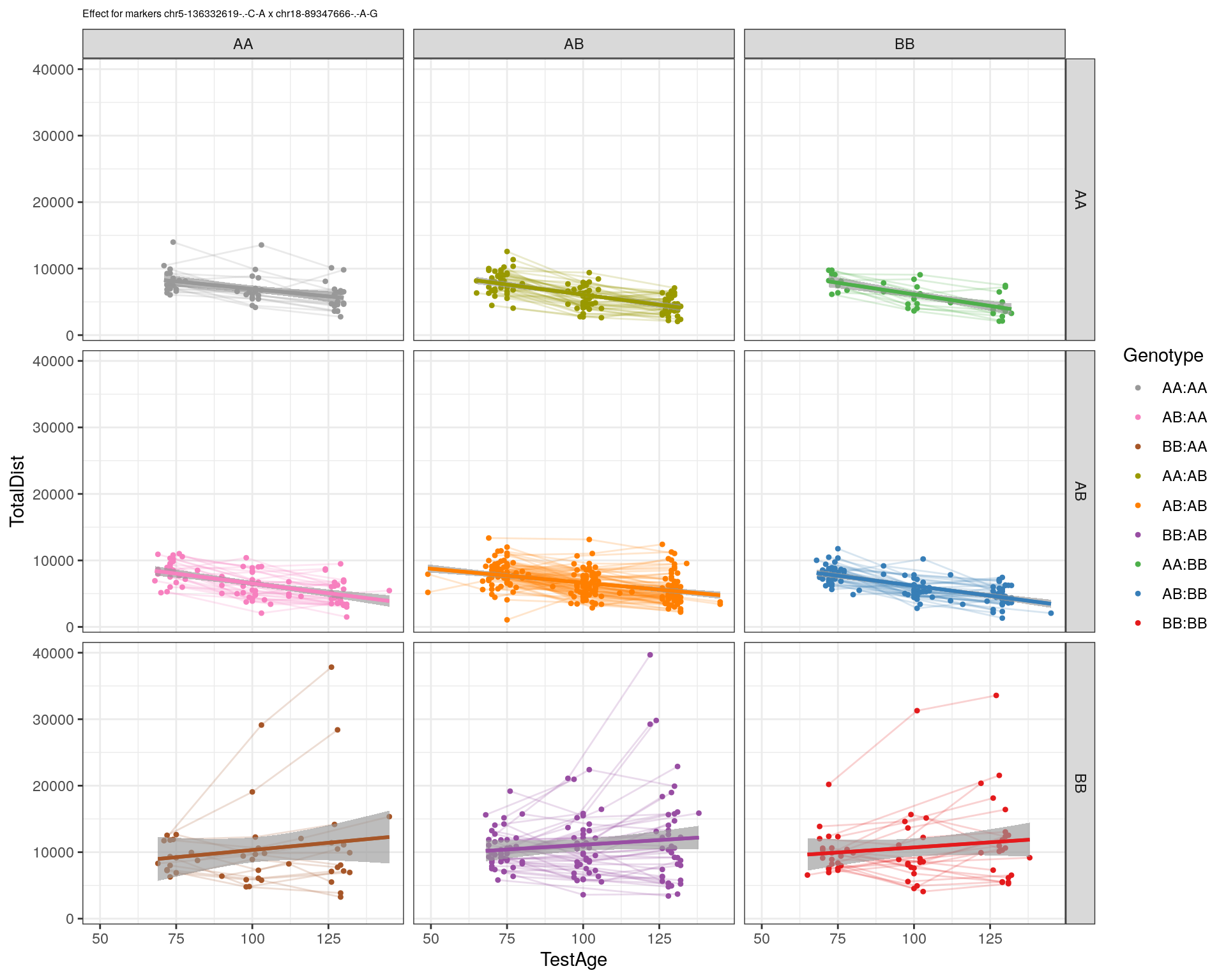
[1] "chr19-29815794-.-A-T"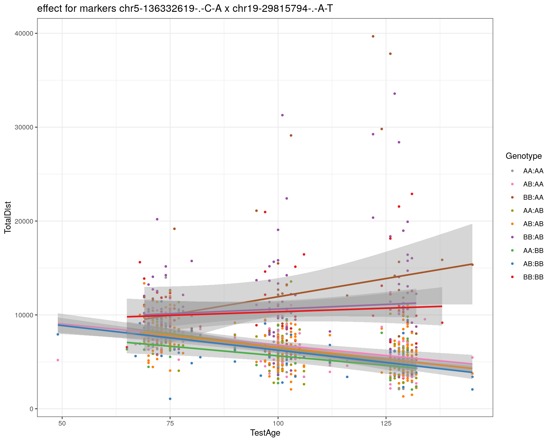
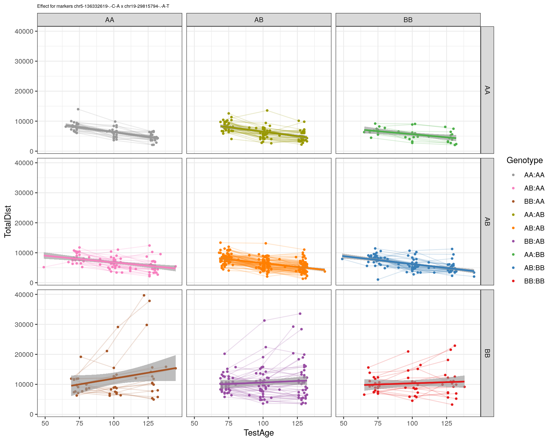
[1] "chr19-45958839-.-A-T"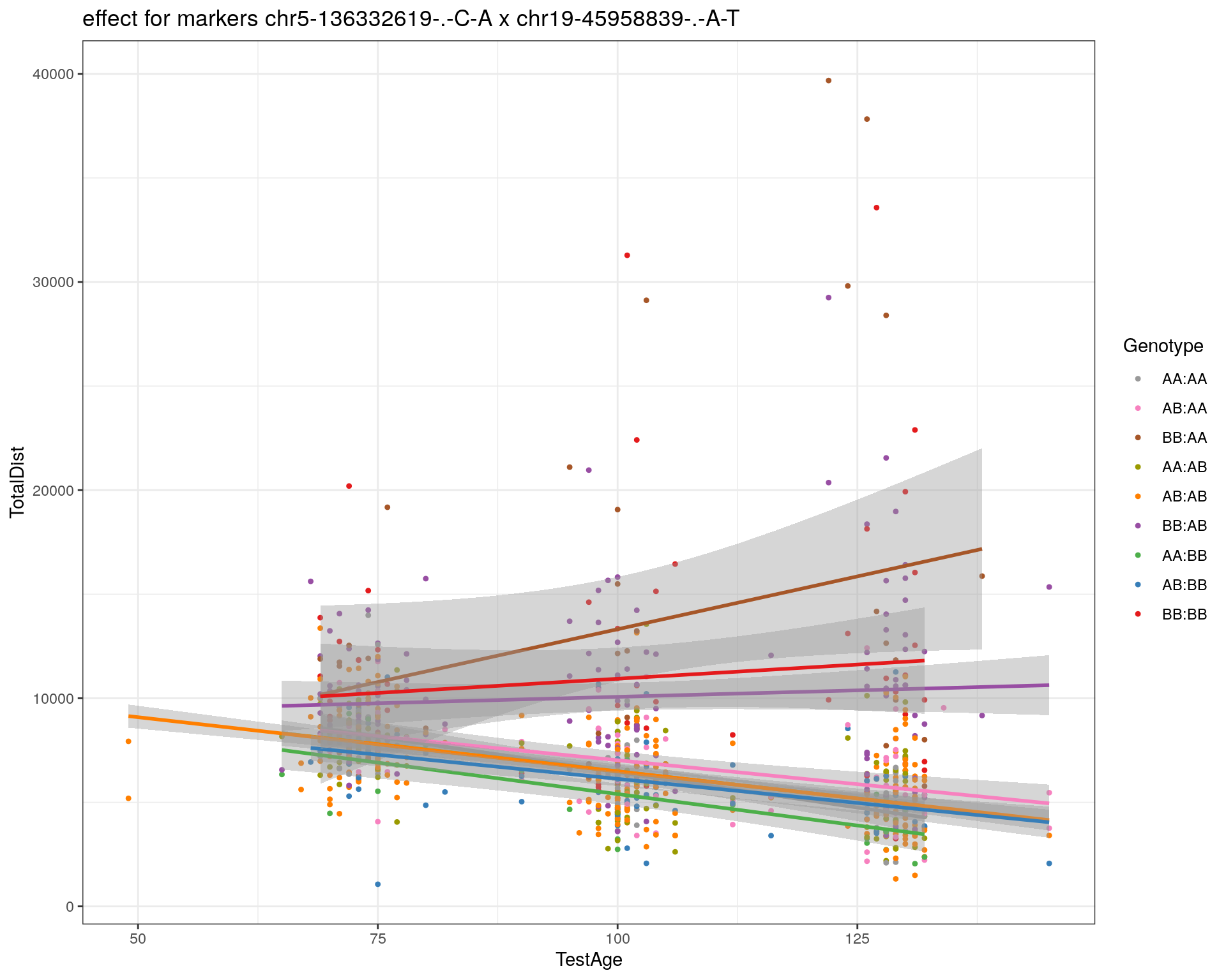
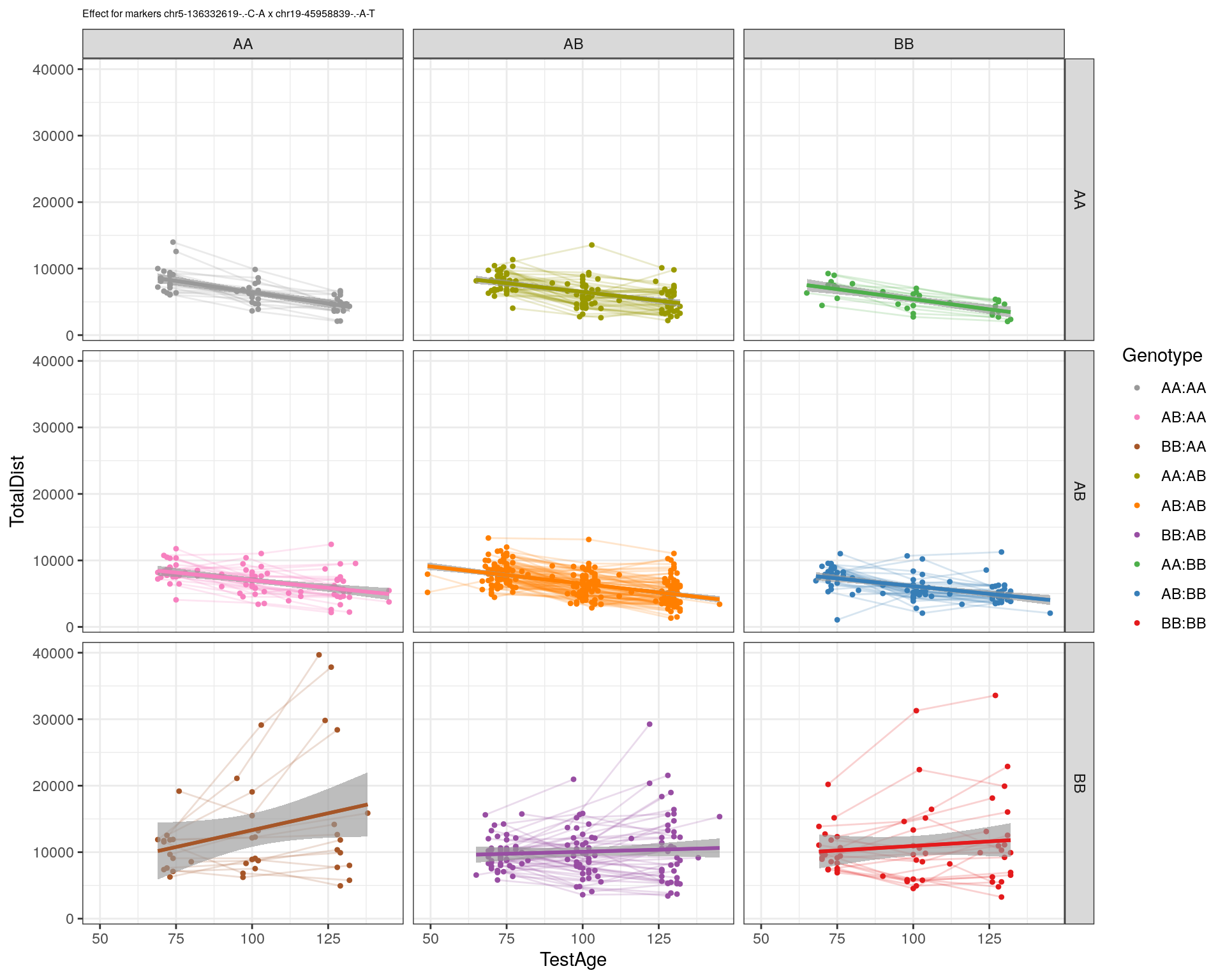
[1] "chr19-53469239-.-A-G"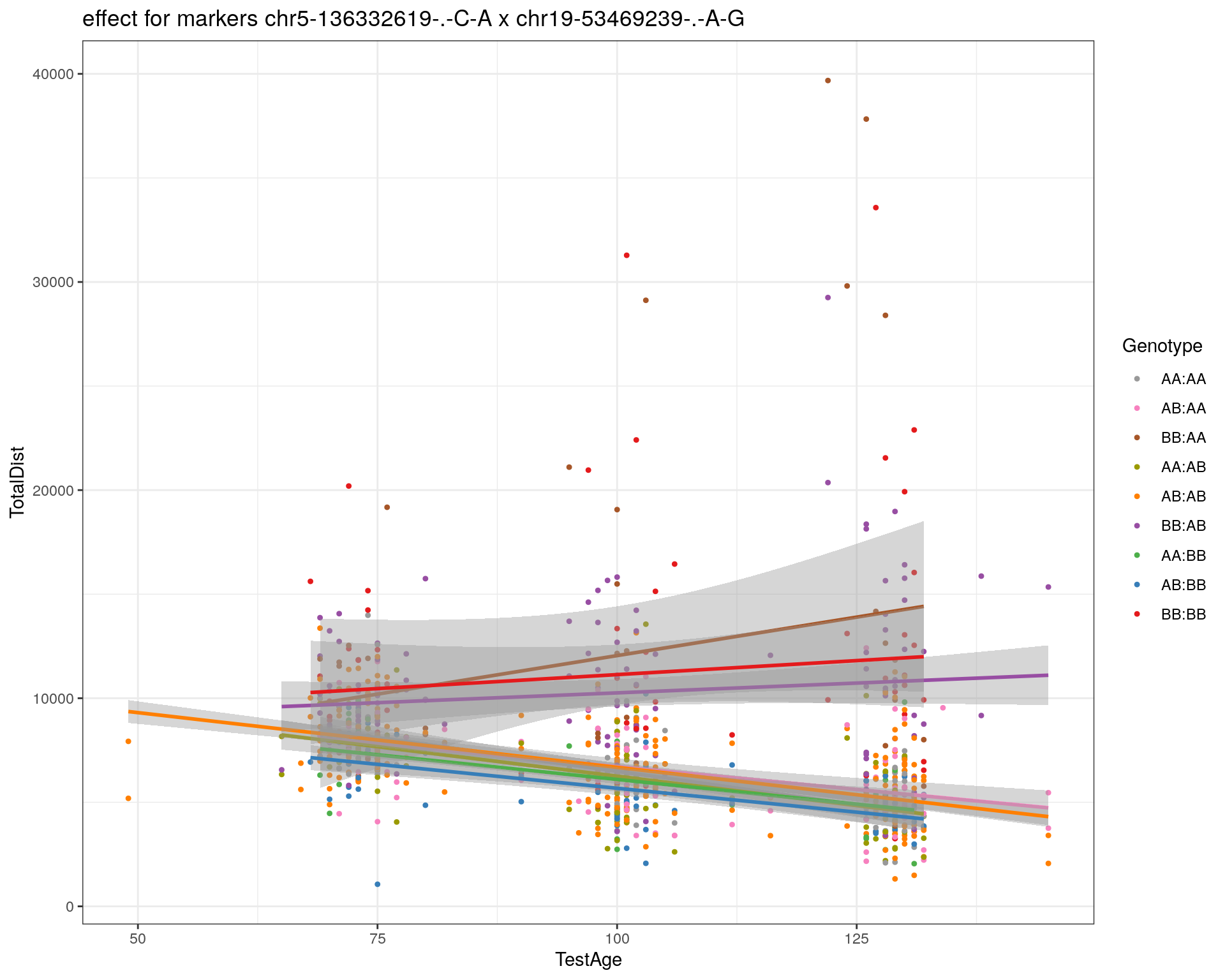
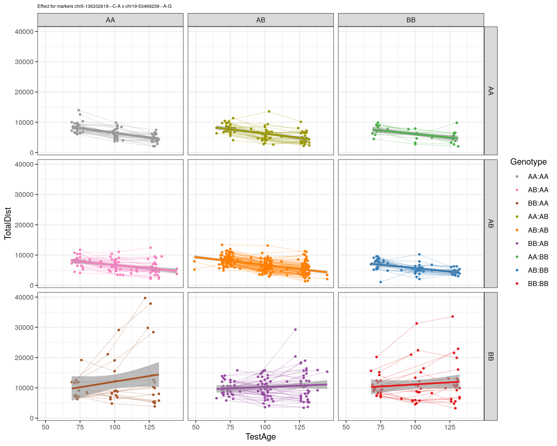
pdf(paste0("output/", paste0("WT144_effect_for_marker_", "_int_chr5-136332619-.-C-A"), ".pdf"))
plot_int_graph(WT144, paste0("WT144_effect_for_marker_", "_int_chr5-136332619-.-C-A"), "chr5-136332619-.-C-A")
[1] "chr1-65643621-.-C-A"[1] "chr1-74679418-.-A-G"[1] "chr1-79823528-.-A-G"[1] "chr1-86851039-.-A-G"[1] "chr1-188155143-.-G-A"[1] "chr2-7018694-.-G-T"[1] "chr2-79706301-.-T-A"[1] "chr2-92367783-.-T-C"[1] "chr2-95118744-.-T-A"[1] "chr2-102169266-.-C-T"[1] "chr2-130405980-.-A-T"[1] "chr2-137498061-.-T-A"[1] "chr2-145128463-.-A-T"[1] "chr3-59218564-.-T-A"[1] "chr3-98881230-.-G-A"[1] "chr3-106985708-.-A-C"[1] "chr3-135614002-.-T-G"[1] "chr3-145286160-.-C-A"[1] "chr3-146750531-.-A-G"[1] "chr3-152699551-.-G-A"[1] "chr4-32821418-.-C-T"[1] "chr5-75264187-.-T-C"[1] "chr5-90233933-.-A-T"[1] "chr5-97607237-.-T-A"[1] "chr5-107507008-.-C-T"[1] "chr5-112799362-.-C-T"[1] "chr5-120660771-.-T-A"[1] "chr5-122167749-.-T-C"[1] "chr5-125153901-.-C-T"[1] "chr5-126058493-.-T-A"[1] "chr5-126551890-.-T-A"[1] "chr5-127565504-.-T-A"[1] "chr5-130394596-.-T-C"[1] "chr5-130943677-.-T-A"[1] "chr5-131298836-.-T-C"[1] "chr5-133052642-.-T-G"[1] "chr5-135960983-.-T-C"[1] "chr5-136332619-.-C-A"[1] "chr5-136844385-.-T-G"[1] "chr5-138956439-.-T-C"[1] "chr5-139706036-.-T-C"[1] "chr5-139891407-.-T-C"[1] "chr5-140071081-.-C-A"[1] "chr7-35061547-.-A-G"[1] "chr7-44272713-.-T-C"[1] "chr7-66785411-.-A-G"[1] "chr7-112510032-.-A-T"[1] "chr8-91986173-.-T-C"[1] "chr8-99395759-.-T-C"[1] "chr8-112465004-.-G-A"[1] "chr9-64698947-.-C-T"[1] "chr9-65857475-.-T-C"[1] "chr9-69415567-.-T-A"[1] "chr9-71739608-.-T-A"[1] "chr9-80465702-.-T-A"[1] "chr10-24134777-.-A-T"[1] "chr11-96730656-.-A-G"[1] "chr12-43136399-.-A-T"[1] "chr12-69197484-.-C-A"[1] "chr12-86851130-.-T-A"[1] "chr12-112415100-.-G-A"[1] "chr13-20165684-.-T-A"[1] "chr13-115031098-.-T-C"[1] "chr14-11709591-.-T-C"[1] "chr14-50642778-.-G-A"[1] "chr14-62407765-.-T-A"[1] "chr14-69691477-.-G-T"[1] "chr15-58605950-.-C-G"[1] "chr15-74727869-.-C-T"[1] "chr16-32593683-.-A-G"[1] "chr16-75648687-.-G-A"[1] "chr17-61305603-.-G-A"[1] "chr17-69219676-.-G-A"[1] "chr18-51300216-.-T-A"[1] "chr18-89347666-.-A-G"[1] "chr19-29815794-.-A-T"[1] "chr19-45958839-.-A-T"[1] "chr19-53469239-.-A-G"dev.off()png
2 Figure panel for publication
# define a function that emits the desired plot
figA <- function() {
  par(
    mar = c(3, 5, 1, 1),
    mgp = c(2, 1, 0)
  )
  #plot phenotypes: slope and totaldistance3
  plot(out.mr[[9]], col= "blue", ylim = c(0, 30), ylab = "LOD score")
  plot(out.mr[[5]], col=  "green", add=TRUE)
  abline(h=3.2, col="red", lty=2, lwd=3)
  # Add a legend
  legend("topright",
         legend=c("Slope", "Total distance traveled"),
         col=c("blue", "green"), lty=1, cex=0.8)
}

figB <- function() {
  par(
    mar = c(3, 5, 1, 0.5),
    mgp = c(2, 1, 0)
  )
  #only at chr 5 and 14
  #plot phenotypes: slope and totaldistance3
  plot(out.mr[[9]], col= "blue", ylim = c(0, 30), ylab = "LOD score", chr = c(5), main = "QTL Interval Chr 5")
  plot(out.mr[[5]], col=  "green", add=TRUE, chr = c(5))
  abline(h=3.2, col="red", lty=2, lwd=3)
  #abline(v= 76.0, col="black", lty=2, lwd=1)
  text(75.5, 29, "5@76.0", cex = 0.75)
  segments(x0 = 76,
         x1 = 76,
         y0 = 0,
         y1 = 28,
         col="black", lty=2, lwd=1)
    segments(x0 = 72.40574,
         x1 = 77.76853,
         y0 = 2,
         y1 = 2,
         col="black", lty=1, lwd=2)
    segments(x0 = 72.40574,
         x1 = 72.40574,
         y0 = 1.85,
         y1 = 2.15,
         col="black", lty=1, lwd=2)
    segments(x0 = 77.76853,
         x1 = 77.76853,
         y0 = 1.85,
         y1 = 2.15,
         col="black", lty=1, lwd=2)
    text(63, 1, "1.5-LOD interval", cex = 0.75)
  # Add a legend
  # legend("topright",
  #        legend=c("Slope", "Total Distance traveled"),
  #        col=c("blue", "green"), lty=1, cex=0.8)
}


figC <- function() {
  par(
    mar = c(3, 5, 1, 0.5),
    mgp = c(2, 1, 0)
  )
  #only at chr 5 and 14
  #plot phenotypes: slope and totaldistance3
plot(out.mr[[9]], col= "blue", ylim = c(0, 30), ylab = "LOD score", chr = c(14), main = "QTL Interval Chr 14")
plot(out.mr[[5]], col=  "green", add=TRUE, chr = c(14))
abline(h=3.2, col="red", lty=2, lwd=3)
#abline(v= 76.0, col="black", lty=2, lwd=1)
text(34, 7, "14@36.1", cex = 0.75)
segments(x0 = 36.07219,
         x1 = 36.07219,
         y0 = 0,
         y1 = 6.4,
         col="black", lty=2, lwd=1)
segments(x0 = 26.14,
         x1 = 36.07219,
         y0 = 2,
         y1 = 2,
         col="black", lty=1, lwd=2)
segments(x0 = 26.14,
         x1 = 26.14,
         y0 = 1.85,
         y1 = 2.15,
         col="black", lty=1, lwd=2)
segments(x0 = 36.07219,
         x1 = 36.07219,
         y0 = 1.85,
         y1 = 2.15,
         col="black", lty=1, lwd=2)
text(29.5, 1, "1.5-LOD interval", cex = 0.75)
  # Add a legend
  # legend("topright",
  #        legend=c("Slope", "Total Distance traveled"),
  #        col=c("blue", "green"), lty=1, cex=0.8)
}


figD <- function() {
 par(mar = c(5, 5, 1, 0.5),
     mgp = c(3, 0.8, 0))
  #interaction_effect for slope
  effectplot(WT144, main = "",
             mname1 = marker[[1]],
             mname2 = marker[[2]], ylab = "Total distance traveled",
             xlab = marker[[2]],
             pheno.col = 11, add.legend=F)
  # Add a legend
  legend("topleft", legend=c("AA", "AB", "BB"), title = marker[[1]],
       col=c("black","red", "blue"), pch = 1, lty=1, cex=0.8)
}

figE <- function() {
  par(
    mar = c(3, 5, 1, 1),
    mgp = c(3, 1, 0)
  )
  #interaction_effect for slope
  effectplot(WT144, main = "",
             mname1 = marker[[1]],
             mname2 = marker[[2]], ylab = "Slope",xlab = marker[[2]],
             pheno.col = 15, add.legend=F)
}

cross = WT144
basem = "chr5-136332619-.-C-A"

# Plot the Dist vs age, separate by genotype for each marker
allphen <- cross$pheno
allgeno <- as.data.frame(pull.geno(cross))
rownames(allgeno) <- cross$pheno$AnimalName
allphen <- merge(allphen, allgeno, by.x="AnimalName", by.y="row.names", all.x=TRUE)
#pdf(paste0("output/", name, ".pdf"))
#for (mar in colnames(allgeno)){
mar = "chr14-69691477-.-G-T"
  print(mar)
[1] "chr14-69691477-.-G-T" subplot <- allphen[!is.na(allphen[,mar, drop=FALSE]),] %>%
pivot_longer(cols = starts_with("TestAge_"), names_to="test.no", values_to = "Age") %>%
separate(test.no, c("empty1", "test1")) %>%
pivot_longer(cols = starts_with("TotalDist_"), names_to="test.no.2", values_to = "Dist") %>%
separate(test.no.2, c("empty2", "test2")) %>% filter(test1==test2)
subplot <- as.data.frame(subplot)
subplot$interactions <- factor(subplot[, basem] + subplot[, mar]*3)
# 1:1 -> 4 1:2 -> 7 1:3 -> 10
# 2:1 -> 5 2:2 -> 8 2:3 -> 11
# 3:1 -> 6 3:2 -> 9 3:3 -> 12
itypes <- c(1,2,3,"AA:AA", "AB:AA", "BB:AA",
"AA:AB", "AB:AB", "BB:AB",
"AA:BB", "AB:BB", "BB:BB")
levels(subplot$interactions) <- itypes[as.integer(levels(subplot$interactions))]
#replaces 1 2 and 3 as AA, AB and BB
subplot[, basem][subplot[, basem] == 1] <- "AA"
subplot[, basem][subplot[, basem] == 2] <- "AB"
subplot[, basem][subplot[, basem] == 3] <- "BB"
subplot[, mar][subplot[, mar] == 1] <- "AA"
subplot[, mar][subplot[, mar] == 2] <- "AB"
subplot[, mar][subplot[, mar] == 3] <- "BB"
p1 <- ggplot(subplot, aes(Age, Dist, color=interactions, group=interactions)) +
geom_point(shape = 20, size=0.75) +
#scale_color_discrete("Genotype") +
labs(color = "Genotype") +
ylab("TotalDist") +
xlab("Test Age") +
#scale_color_brewer(palette = "Set1") +
scale_color_manual(breaks = c("AA:AA", "AB:AA", "BB:AA", "AA:AB",
"AB:AB", "BB:AB", "AA:BB", "AB:BB", "BB:BB"),
#values = RColorBrewer::brewer.pal(9, "Set1")[9:1]) +
values = c("#999999", "#F781BF", "#A65628","#9a9a00", "#FF7F00", "#984EA3", "#4DAF4A", "#377EB8", "#E41A1C")) +
stat_smooth(method="lm", show.legend = FALSE, formula = y~x) +
labs(title=paste0("effect for markers ", basem, " x ", mar)) +
theme_bw()
print(p1)Warning: Removed 29 rows containing non-finite values (stat_smooth).Warning: Removed 29 rows containing missing values (geom_point).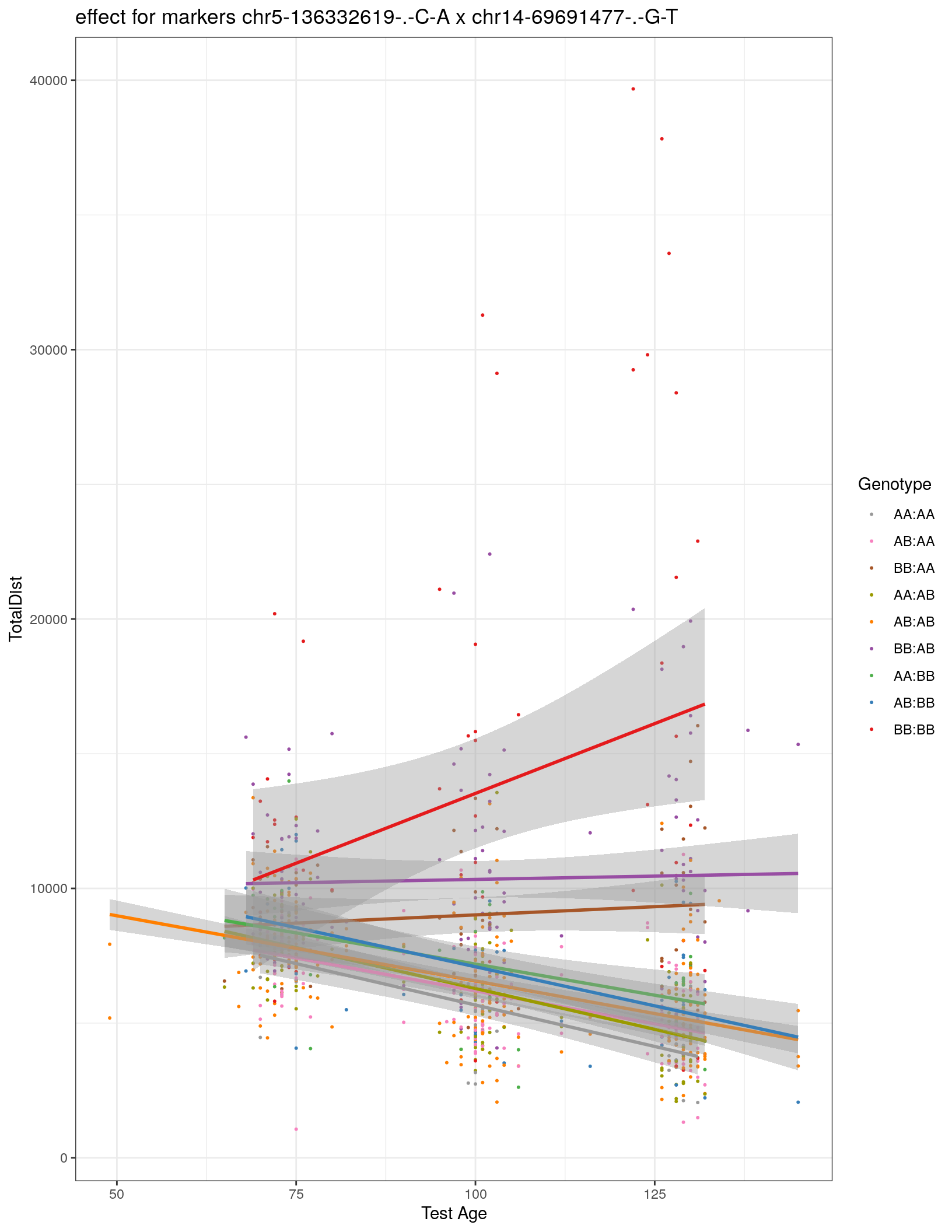
  p2 <- ggplot(subplot, aes(Age, Dist, color=interactions, group=interactions)) +
    geom_point(shape = 20, show.legend = FALSE) +
    geom_line(aes(group = AnimalName, color = interactions), show.legend = FALSE, alpha = 0.2) +
    geom_smooth(method='lm', formula= y~x, show.legend = FALSE, size = 1) +
    #scale_color_discrete("Genotype") +
    labs(color = "Genotype") +
    ylab("Total distance traveled / Chr14") +
    xlab("Test age / Chr5") +
    #scale_color_brewer(palette = "Set1") +
    scale_color_manual(breaks = c("AA:AA", "AB:AA", "BB:AA", "AA:AB",
                                  "AB:AB", "BB:AB", "AA:BB", "AB:BB", "BB:BB"),
                       #values = RColorBrewer::brewer.pal(9, "Set1")[9:1]) +
                       values = c("#999999", "#F781BF", "#A65628","#9a9a00", "#FF7F00", "#984EA3", "#4DAF4A", "#377EB8", "#E41A1C")) +
    stat_smooth(method="lm", show.legend = FALSE, formula = y~x) +
    labs(title=paste0("Interaction effect between Chr5 and Chr14")) +
    facet_grid(rows = vars(subplot[, basem]), cols = vars(subplot[, mar])) +
    theme_bw() +
    theme(panel.grid.major = element_blank(), panel.grid.minor = element_blank()) +
    theme(plot.title = element_text(hjust = 0.5))
  print(p2)
Warning: Removed 29 rows containing non-finite values (stat_smooth).Warning: Removed 29 rows containing non-finite values (stat_smooth).Warning: Removed 29 rows containing missing values (geom_point).Warning: Removed 29 row(s) containing missing values (geom_path).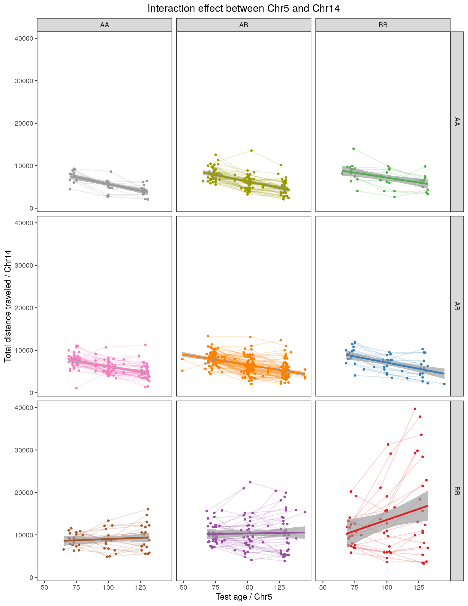
pp2 = plot_grid(figB, figC, labels = c("B", "C"), align = 'h', ncol=2)
pp3 = plot_grid(figD, p2, labels = c("D", "E"), align = 'h',ncol=2)
Warning: Removed 29 rows containing non-finite values (stat_smooth).Warning: Removed 29 rows containing non-finite values (stat_smooth).Warning: Removed 29 rows containing missing values (geom_point).Warning: Removed 29 row(s) containing missing values (geom_path).Warning: Graphs cannot be horizontally aligned unless the axis parameter is set.
Placing graphs unaligned.pdf("output/figure_panel.pdf", width = 8.5, height = 11)
plot_grid(figA, labels = c('A', ''),
  pp2,
  pp3,
  nrow = 3
)
dev.off()png
2 plot_grid(figA, labels = c('A', ''),
pp2,
pp3,
nrow = 3
)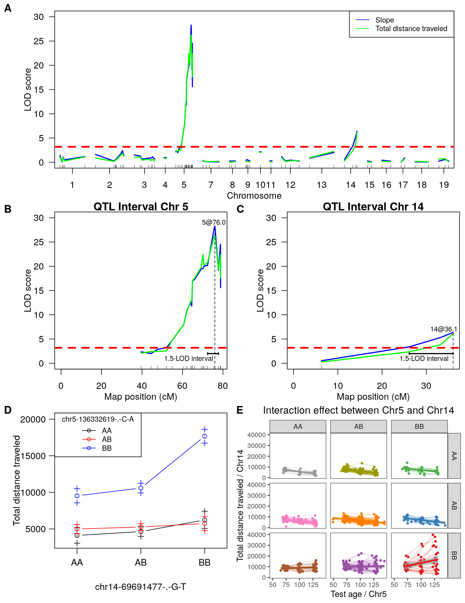
sessionInfo()R version 4.0.3 (2020-10-10)
Platform: x86_64-pc-linux-gnu (64-bit)
Running under: Ubuntu 20.04.2 LTS
Matrix products: default
BLAS/LAPACK: /usr/lib/x86_64-linux-gnu/openblas-pthread/libopenblasp-r0.3.8.so
locale:
[1] LC_CTYPE=en_US.UTF-8 LC_NUMERIC=C
[3] LC_TIME=en_US.UTF-8 LC_COLLATE=en_US.UTF-8
[5] LC_MONETARY=en_US.UTF-8 LC_MESSAGES=C
[7] LC_PAPER=en_US.UTF-8 LC_NAME=C
[9] LC_ADDRESS=C LC_TELEPHONE=C
[11] LC_MEASUREMENT=en_US.UTF-8 LC_IDENTIFICATION=C
attached base packages:
[1] stats graphics grDevices utils datasets methods base
other attached packages:
[1] cowplot_1.1.1 qtl2_0.24 lmerTest_3.1-3 lme4_1.1-26
[5] Matrix_1.3-2 forcats_0.5.1 stringr_1.4.0 dplyr_1.0.4
[9] purrr_0.3.4 readr_1.4.0 tidyr_1.1.2 tibble_3.0.6
[13] tidyverse_1.3.0 qtlcharts_0.12-10 qtl_1.47-9 gridExtra_2.3
[17] ggplot2_3.3.3 workflowr_1.6.2
loaded via a namespace (and not attached):
[1] nlme_3.1-152 fs_1.5.0 lubridate_1.7.9.2
[4] bit64_4.0.5 RColorBrewer_1.1-2 httr_1.4.2
[7] rprojroot_2.0.2 numDeriv_2016.8-1.1 tools_4.0.3
[10] backports_1.2.1 R6_2.5.0 mgcv_1.8-34
[13] DBI_1.1.1 colorspace_2.0-0 withr_2.4.1
[16] tidyselect_1.1.0 bit_4.0.4 compiler_4.0.3
[19] git2r_0.28.0 cli_2.3.0 rvest_0.3.6
[22] xml2_1.3.2 labeling_0.4.2 scales_1.1.1
[25] digest_0.6.27 minqa_1.2.4 rmarkdown_2.6
[28] pkgconfig_2.0.3 htmltools_0.5.1.1 highr_0.8
[31] dbplyr_2.1.0 fastmap_1.1.0 rlang_1.0.2
[34] readxl_1.3.1 rstudioapi_0.13 RSQLite_2.2.3
[37] gridGraphics_0.5-1 farver_2.0.3 generics_0.1.0
[40] jsonlite_1.7.2 magrittr_2.0.1 Rcpp_1.0.6
[43] munsell_0.5.0 lifecycle_1.0.0 stringi_1.5.3
[46] whisker_0.4 yaml_2.2.1 MASS_7.3-53.1
[49] grid_4.0.3 blob_1.2.1 parallel_4.0.3
[52] promises_1.2.0.1 crayon_1.4.1 lattice_0.20-41
[55] haven_2.3.1 splines_4.0.3 hms_1.0.0
[58] knitr_1.31 pillar_1.4.7 boot_1.3-27
[61] reprex_1.0.0 glue_1.4.2 evaluate_0.14
[64] data.table_1.13.6 modelr_0.1.8 vctrs_0.3.6
[67] nloptr_1.2.2.2 httpuv_1.5.5 cellranger_1.1.0
[70] gtable_0.3.0 assertthat_0.2.1 cachem_1.0.4
[73] xfun_0.21 broom_0.7.4 later_1.1.0.1
[76] memoise_2.0.0 statmod_1.4.35 ellipsis_0.3.1