QTL analysis for Crichton final

workflowr

• Summary
• Checks
• Past versions

Last updated: 2023-02-04

Checks: 7 0

Knit directory: QTL_analysis_for_Crichton/

This reproducible R Markdown analysis was created with workflowr (version 1.6.2). The Checks tab describes the reproducibility checks that were applied when the results were created. The Past versions tab lists the development history.

---

R Markdown file: up-to-date

Great! Since the R Markdown file has been committed to the Git repository, you know the exact version of the code that produced these results.

Environment: empty

Great job! The global environment was empty. Objects defined in the global environment can affect the analysis in your R Markdown file in unknown ways. For reproduciblity it’s best to always run the code in an empty environment.

Seed: set.seed(20221224)

The command set.seed(20221224) was run prior to running the code in the R Markdown file. Setting a seed ensures that any results that rely on randomness, e.g. subsampling or permutations, are reproducible.

Session information: recorded

Great job! Recording the operating system, R version, and package versions is critical for reproducibility.

Cache: none

Nice! There were no cached chunks for this analysis, so you can be confident that you successfully produced the results during this run.

File paths: relative

Great job! Using relative paths to the files within your workflowr project makes it easier to run your code on other machines.

Repository version: ff93680

Great! You are using Git for version control. Tracking code development and connecting the code version to the results is critical for reproducibility.

The results in this page were generated with repository version ff93680. See the Past versions tab to see a history of the changes made to the R Markdown and HTML files.

Note that you need to be careful to ensure that all relevant files for the analysis have been committed to Git prior to generating the results (you can use wflow_publish or wflow_git_commit). workflowr only checks the R Markdown file, but you know if there are other scripts or data files that it depends on. Below is the status of the Git repository when the results were generated:

Ignored files:
    Ignored:    .Rhistory
    Ignored:    .Rproj.user/

Untracked files:
    Untracked:  output/WT144_effect_for_marker__int_chr5-136332619-.-C-A.pdf
    Untracked:  output/WT144_effect_for_marker_plots_TotalDist_vs_TestAge_by_marker.pdf
    Untracked:  output/WT144_plot-Intercept.pdf
    Untracked:  output/WT144_plot-Slope.pdf
    Untracked:  output/WT144_plot-TestAge.x.pdf
    Untracked:  output/WT144_plot-TestAge.y.pdf
    Untracked:  output/WT144_plot-TotalDist_1.pdf
    Untracked:  output/WT144_plot-TotalDist_2.pdf
    Untracked:  output/WT144_plot-TotalDist_3.pdf
    Untracked:  output/WT144_plot-base.x.pdf
    Untracked:  output/WT144_plot-base.y.pdf
    Untracked:  output/figure_panel.pdf
    Untracked:  output/qtl.out.obj.mixedmodel.RData
    Untracked:  output/qtl.out.obj.mixedmodel.final.RData

Unstaged changes:
    Modified:   analysis/workflow_proc.R

Note that any generated files, e.g. HTML, png, CSS, etc., are not included in this status report because it is ok for generated content to have uncommitted changes.

---

These are the previous versions of the repository in which changes were made to the R Markdown (analysis/QTL_analysis_for_Crichton_final.Rmd) and HTML (docs/QTL_analysis_for_Crichton_final.html) files. If you’ve configured a remote Git repository (see ?wflow_git_remote), click on the hyperlinks in the table below to view the files as they were in that past version.

File	Version	Author	Date	Message
Rmd	ff93680	xhyuo	2023-02-04	change figure panel
html	2470aab	xhyuo	2022-12-24	Build site.
Rmd	92ecd1d	xhyuo	2022-12-24	First build

---

Library

library(ggplot2)
library(gridExtra)
library(qtl)
library(qtlcharts)
library(tidyverse)
library(lme4)
library(lmerTest)
library(qtl2)
library(cowplot)

Load qtl data and plot summary

WT144 <- read.cross(format = "csv", file = "data/WT144_GBS_Rqtl_input.csv", genotypes = c("A", "H", "B"))

 --Read the following data:
     309  individuals
     225  markers
     11  phenotypes
 --Cross type: f2 

chror <- as.character(1:19)
WT144$geno <- WT144$geno[chror]
summary(WT144)

    F2 intercross

    No. individuals:    309 

    No. phenotypes:     11 
    Percent phenotyped: 100 100 100 99.7 100 100 99.7 90.9 100 99.7 90.9 

    No. chromosomes:    19 
        Autosomes:      1 2 3 4 5 6 7 8 9 10 11 12 13 14 15 16 17 18 19 

    Total markers:      225 
    No. markers:        18 23 17 15 46 1 19 4 8 3 5 18 11 10 2 4 7 2 12 
    Percent genotyped:  85 
    Genotypes (%):      AA:40.6  AB:46.9  BB:12.5  not BB:0.0  not AA:0.0 

plotMissing(WT144, main="")

#drop.nullmarkers
WT144 <- drop.nullmarkers(WT144)
plotMissing(WT144, main="")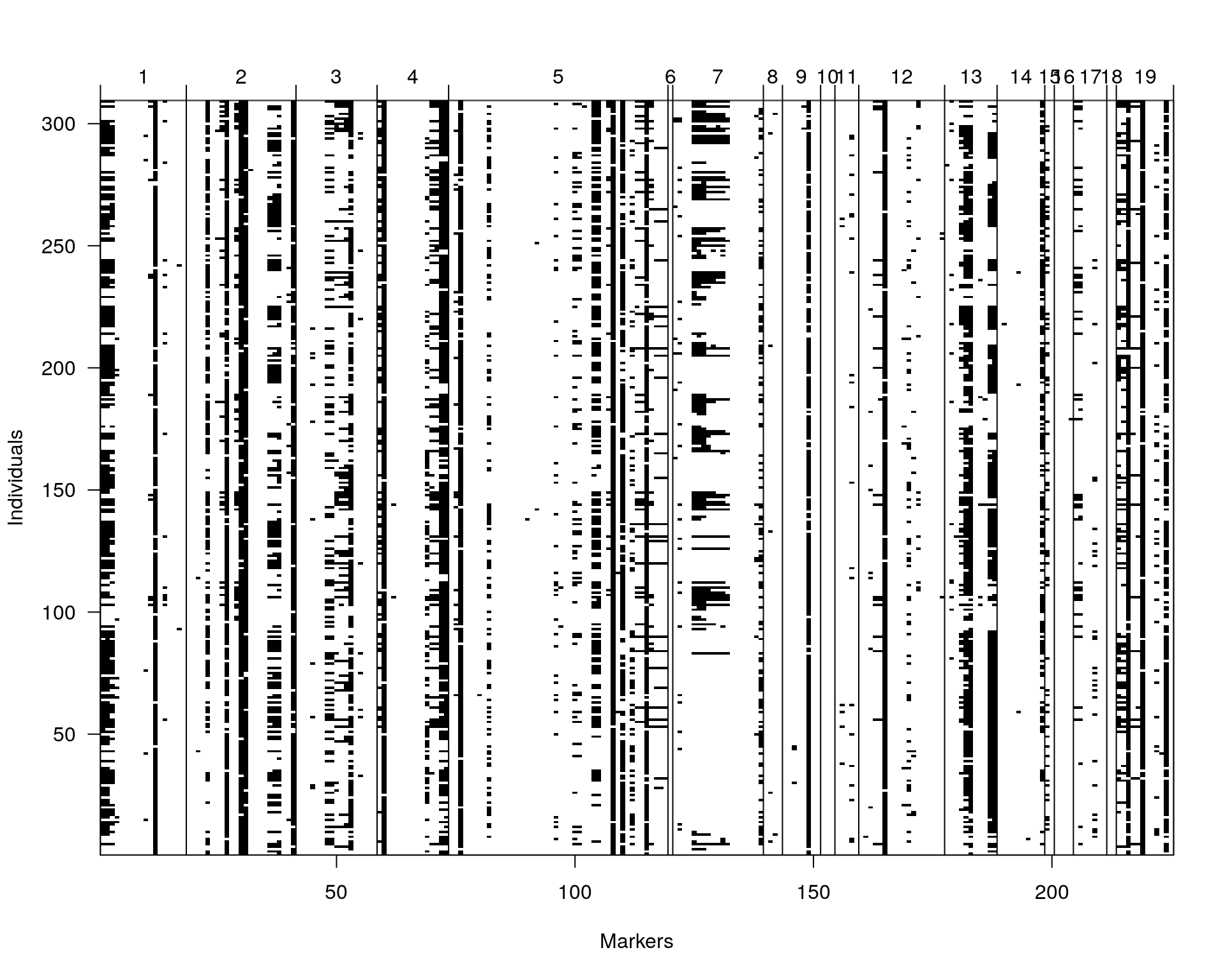

Past versions of “Load qtl data and plot summary-1.png”

Version	Author	Date
2470aab	xhyuo	2022-12-24

Genotype_distribution_pre

# Plot the distribution of homo/hetero for each marker
af <- NULL
for (chr in names(WT144$geno)){
  af <- rbind(af, data.frame(chr=chr,
                             A=colSums(WT144$geno[[chr]]$data == 1, na.rm = T),
                             H=colSums(WT144$geno[[chr]]$data == 2, na.rm = T),
                             B=colSums(WT144$geno[[chr]]$data == 3, na.rm = T),
                             N=colSums(is.na(WT144$geno[[chr]]$data))))
}
af$chr <- factor(af$chr, levels = names(WT144$geno))
af$ID <- 1:nrow(af)
#plot
genotype_distribution_pre <- ggplot(af) + 
  geom_point(aes(ID, A), color = "red") + 
  geom_point(aes(ID, B), color="purple") + 
  geom_point(aes(ID, H), color="green") + 
  geom_point(aes(ID, N), color="black") + 
  facet_grid(~chr, scales = "free") +
  ylab("Frequency") + 
  theme(text = element_text(size = 14),
        axis.text.x = element_blank(),
        axis.ticks = element_blank())
#
print(genotype_distribution_pre)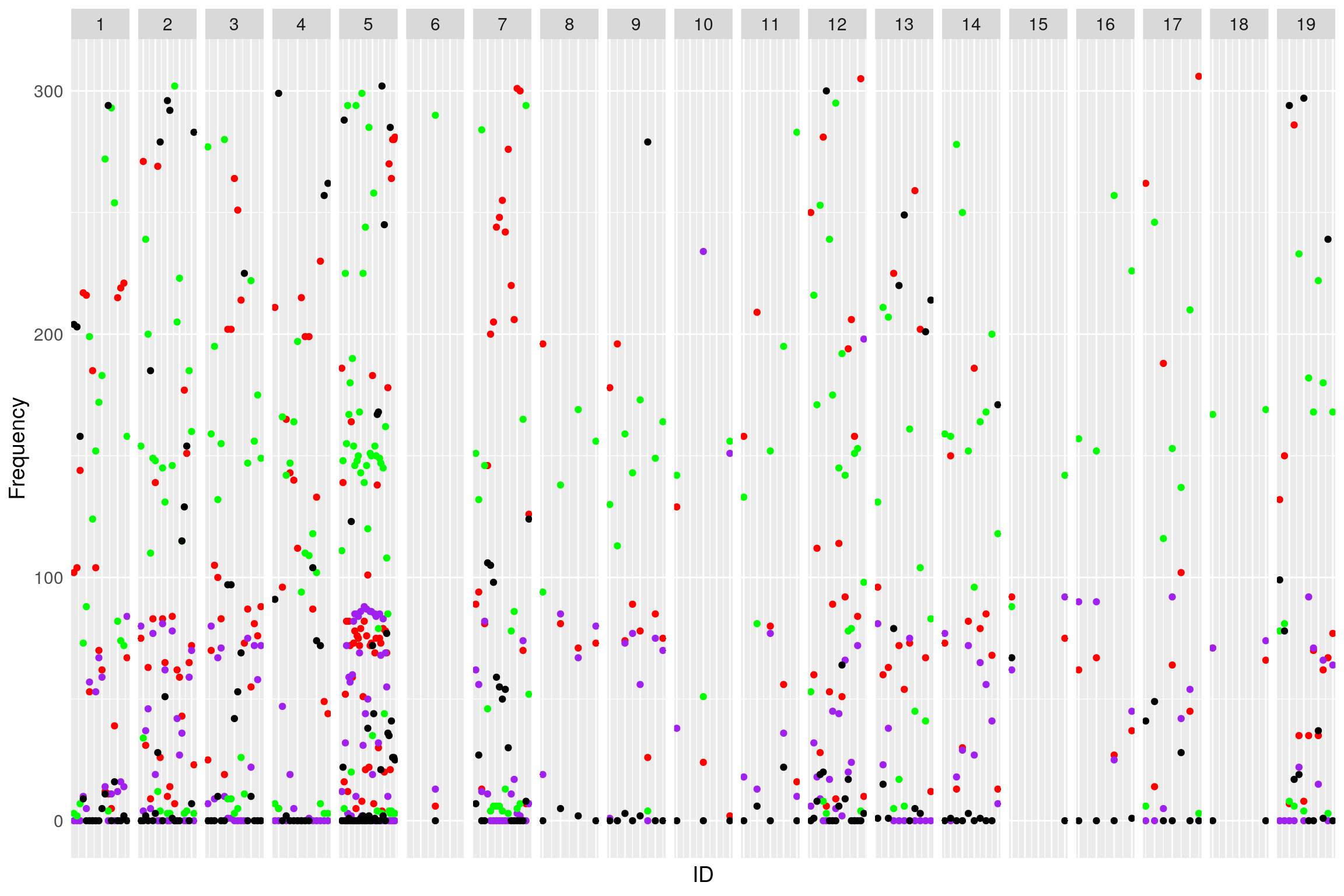

Past versions of Genotype_distribution_pre-1.png

Version	Author	Date
2470aab	xhyuo	2022-12-24

Genotype_distribution_post

# Choose who to drop. I chose A > H/4, B > H/4, H > (A+B)/2
dropm <- rownames(af)[af$A < af$H/4 | af$B < af$H/4 | af$H < (af$A+af$B)/2 | af$N > (af$A+af$B+af$H)] 
WT144 <- drop.markers(WT144, dropm)
# Plot again
af <- NULL
for (chr in names(WT144$geno)){
  af <- rbind(af, data.frame(chr=chr,
                             A=colSums(WT144$geno[[chr]]$data == 1, na.rm = T),
                             H=colSums(WT144$geno[[chr]]$data == 2, na.rm = T),
                             B=colSums(WT144$geno[[chr]]$data == 3, na.rm = T),
                             N=colSums(is.na(WT144$geno[[chr]]$data))))
}
af$chr <- factor(af$chr, levels = names(WT144$geno))
af$ID <- 1:nrow(af)
#plot
genotype_distribution_post <- ggplot(af) + 
  geom_point(aes(ID, A), color = "red") + 
  geom_point(aes(ID, B), color="purple") + 
  geom_point(aes(ID, H), color="green") + 
  geom_point(aes(ID, N), color="black") + 
  facet_grid(~chr, scales = "free") +
  ylab("Frequency") + 
  theme(text = element_text(size = 14),
        axis.text.x = element_blank(),
        axis.ticks = element_blank())

print(genotype_distribution_post)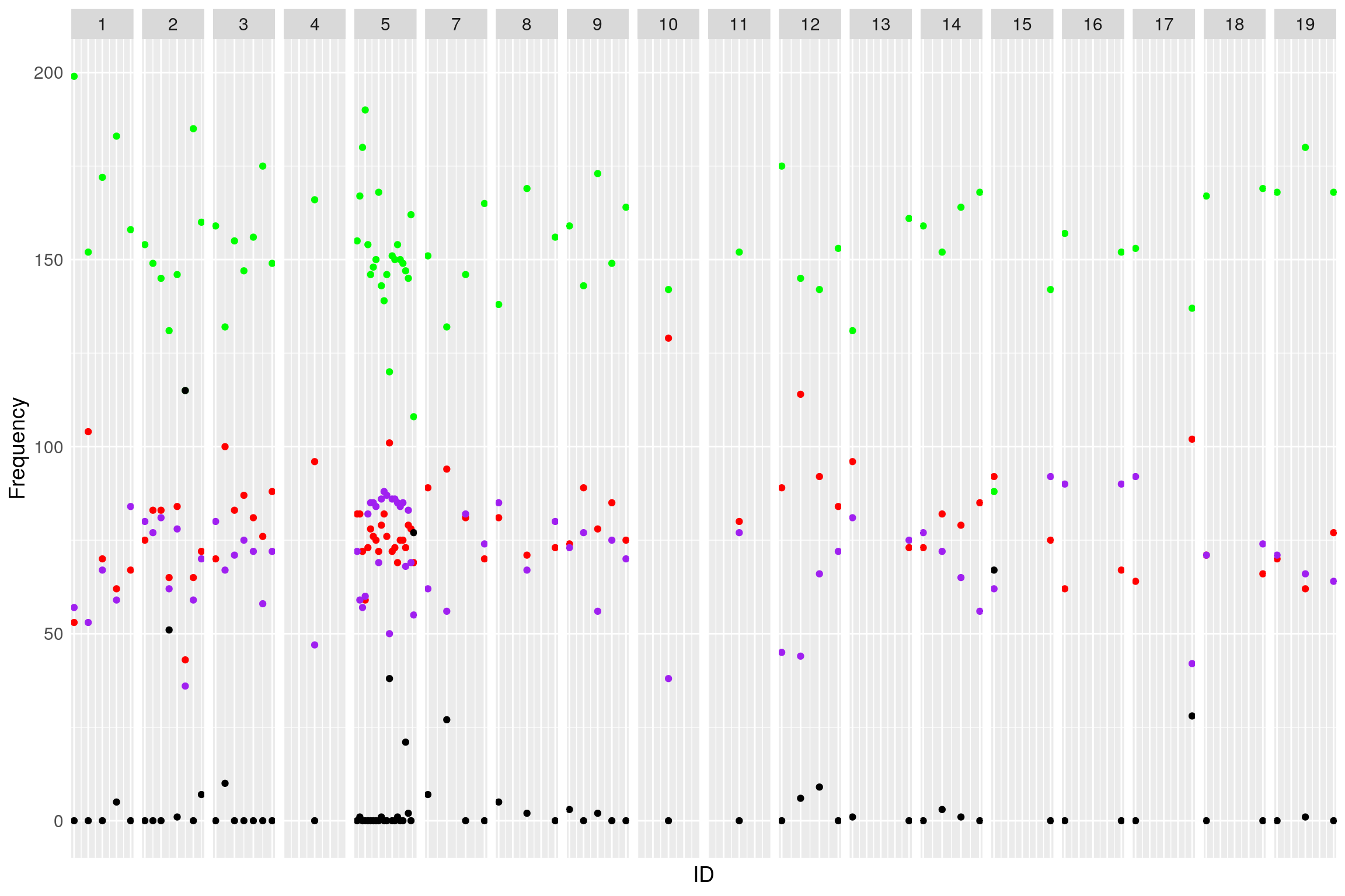

Past versions of Genotype_distribution_post-1.png

Version	Author	Date
2470aab	xhyuo	2022-12-24

plotMap(WT144)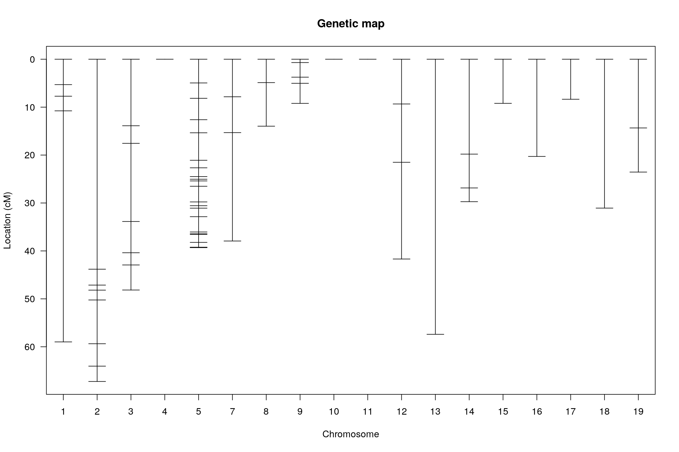

Past versions of Genotype_distribution_post-2.png

Version	Author	Date
2470aab	xhyuo	2022-12-24

Process phenotype on the genotyped animals

#read data Report-12-27-2019.csv and filter to the 309 animals which also have genotypes. 
report <- readr::read_csv("data/Report-12-27-2019.csv") %>% 
  dplyr::select(animal_name, gender, TotalDist, TestAge, test.no) %>%
  dplyr::filter(animal_name %in% WT144$pheno$AnimalName) %>% #filter to the animals with genotypes
  dplyr::mutate(across(c(gender, test.no), as.factor))
#plot TotalDist vs test age among 309 animals
p6 <- ggplot(data = report,  
             mapping = aes(x = TestAge, y = TotalDist, color = test.no)) +
  geom_point(aes(shape=gender)) +
  geom_smooth(method=lm)
print(p6)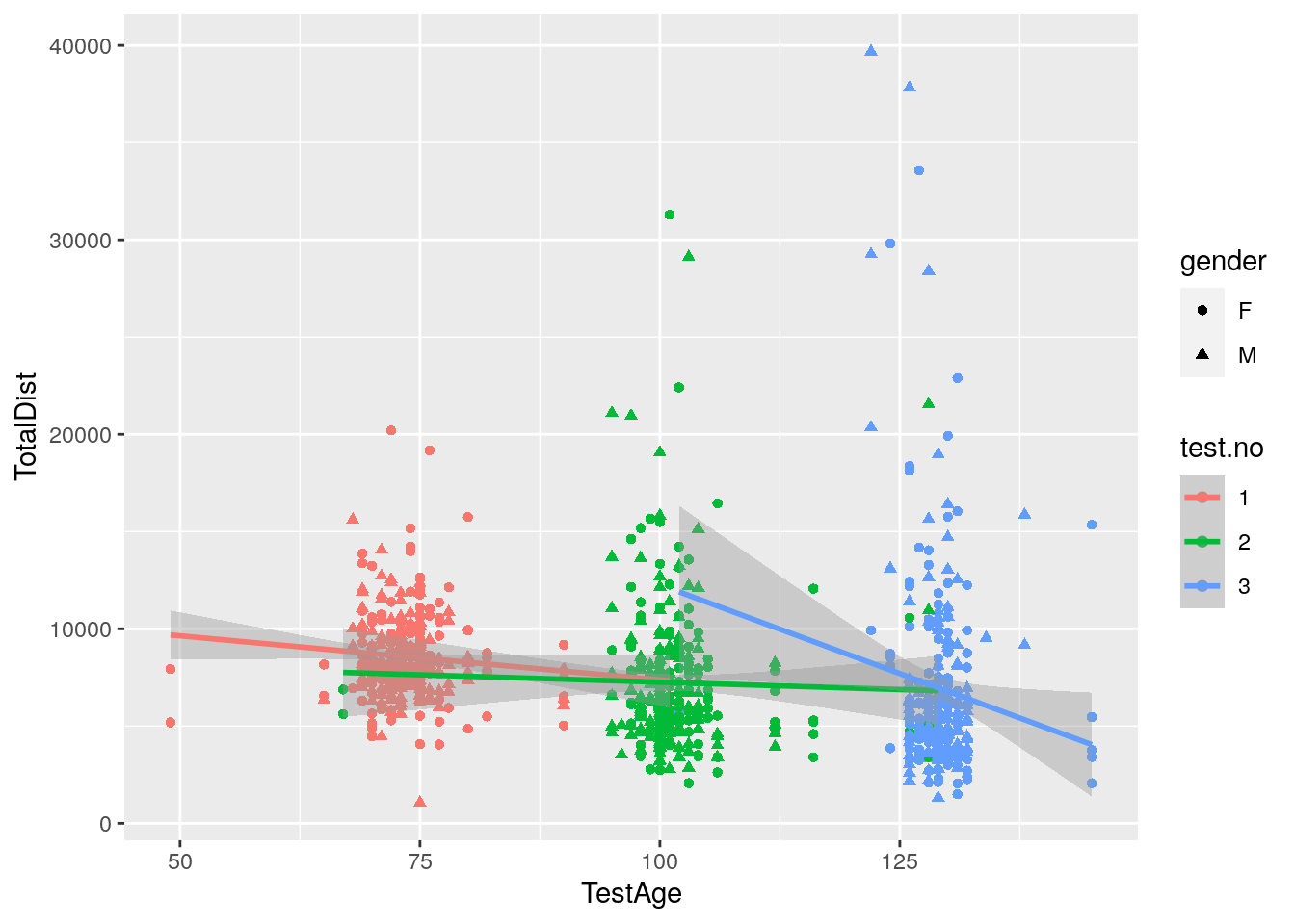

Past versions of “Process phenotype on the genotyped animals-1.png”

Version	Author	Date
2470aab	xhyuo	2022-12-24

#plot TotalDist distribution across test.no among 309 animals
p7 <- ggplot(data = report,  
             mapping = aes(x = test.no, y = TotalDist, color = test.no)) +
  geom_boxplot()
print(p7)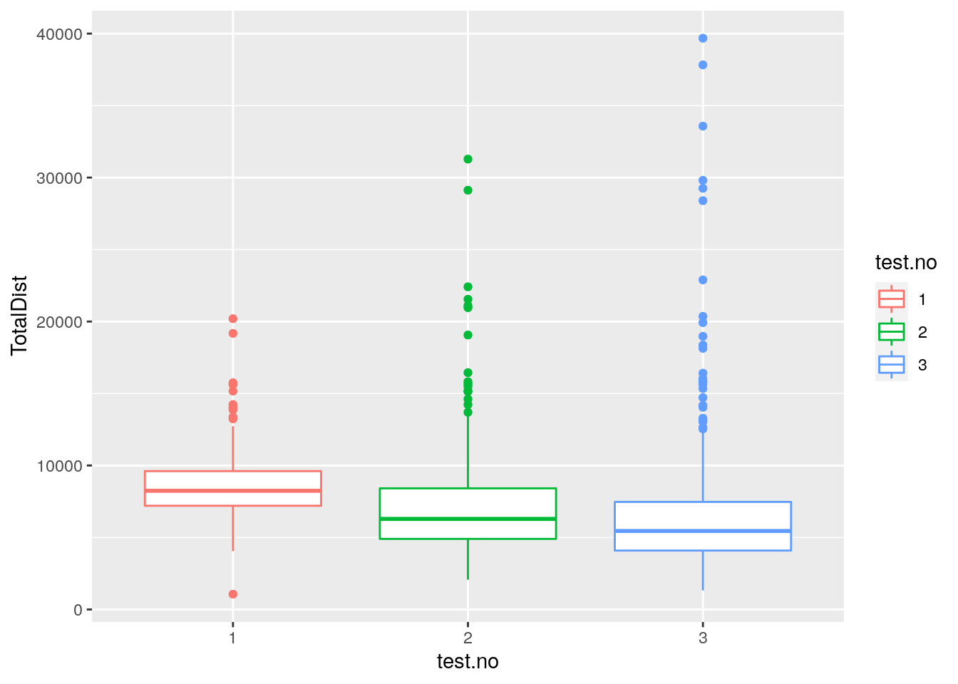

Past versions of “Process phenotype on the genotyped animals-2.png”

Version	Author	Date
2470aab	xhyuo	2022-12-24

#plot histgram for TotalDist among 309 animals
p8 <- ggplot(data = report,  
             mapping = aes(x = TotalDist, fill = test.no)) +
  geom_histogram() +
  facet_grid(test.no ~ .)
print(p8)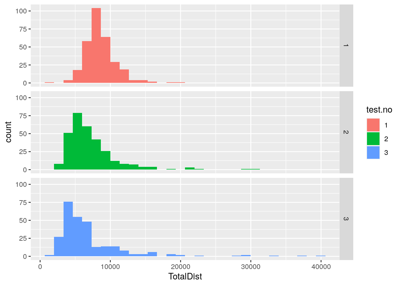

Past versions of “Process phenotype on the genotyped animals-3.png”

Version	Author	Date
2470aab	xhyuo	2022-12-24

#plot histgram for TotalDist for genders with mean lines among 309 animals
p9 <- ggplot(data = report,  
             mapping = aes(x = TotalDist, fill = gender)) +
  geom_histogram()
print(p9)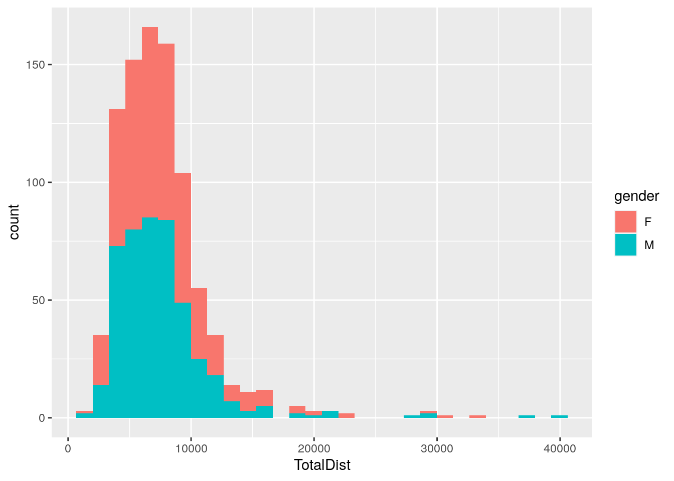

Past versions of “Process phenotype on the genotyped animals-4.png”

Version	Author	Date
2470aab	xhyuo	2022-12-24

#a random intercept for each animal, 
#and a random slope of TestAge for each animal 
#This allows both the intercept and the slope of TestAge to vary across animals
res <- lmer(TotalDist ~ TestAge + (1 + TestAge|animal_name),
              data = report)
summary(res)

Linear mixed model fit by REML. t-tests use Satterthwaite's method [
lmerModLmerTest]
Formula: TotalDist ~ TestAge + (1 + TestAge | animal_name)
   Data: report

REML criterion at convergence: 16596.9

Scaled residuals: 
    Min      1Q  Median      3Q     Max 
-3.5368 -0.4085 -0.0295  0.3694  3.7790 

Random effects:
 Groups      Name        Variance Std.Dev. Corr 
 animal_name (Intercept) 12321442 3510.2        
             TestAge         4265   65.3   -0.96
 Residual                 2173666 1474.3        
Number of obs: 898, groups:  animal_name, 309

Fixed effects:
             Estimate Std. Error        df t value Pr(>|t|)    
(Intercept) 10338.640    302.752   321.518  34.149  < 2e-16 ***
TestAge       -26.522      4.333   317.190  -6.121 2.75e-09 ***
---
Signif. codes:  0 '***' 0.001 '**' 0.01 '*' 0.05 '.' 0.1 ' ' 1

Correlation of Fixed Effects:
        (Intr)
TestAge -0.918
optimizer (nloptwrap) convergence code: 0 (OK)
Model failed to converge with max|grad| = 1.58588 (tol = 0.002, component 1)
Model is nearly unidentifiable: very large eigenvalue
 - Rescale variables?

confint(res, level = 0.95, method = "Wald")

                 2.5 %      97.5 %
.sig01              NA          NA
.sig02              NA          NA
.sig03              NA          NA
.sigma              NA          NA
(Intercept) 9745.25700 10932.02232
TestAge      -35.01462   -18.02879

#there is strong evidence that TestAge significantly decreased TotalDist.

res.std <- resid(res)/sd(resid(res))
plot(res.std, ylab="Standardized Residuals")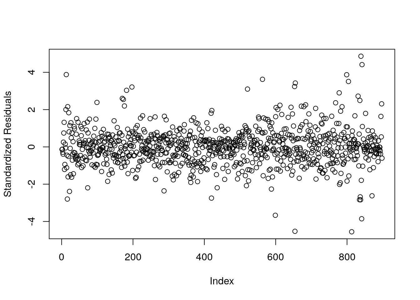

Past versions of “Process phenotype on the genotyped animals-5.png”

Version	Author	Date
2470aab	xhyuo	2022-12-24

ggplot(as.data.frame(res.std), aes(sample = res.std)) +
  geom_qq() +
  geom_qq_line()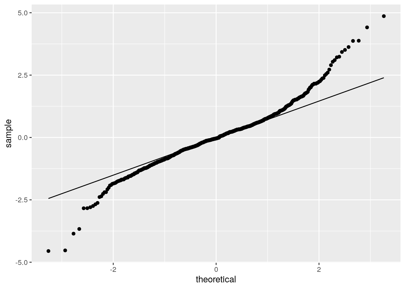

Past versions of “Process phenotype on the genotyped animals-6.png”

Version	Author	Date
2470aab	xhyuo	2022-12-24

#to get the fitted Intercept and Slope
TotalDist_animal <- coef(res)$animal_name
colnames(TotalDist_animal) <- c("Intercept", "Slope")
TotalDist_animal$AnimalName <- rownames(TotalDist_animal)

#add TotalDist_animal to the phenotype df in WT144
WT144$pheno <- left_join(WT144$pheno, TotalDist_animal, by = "AnimalName")
plotPheno(WT144, pheno.col=12, xlab = "")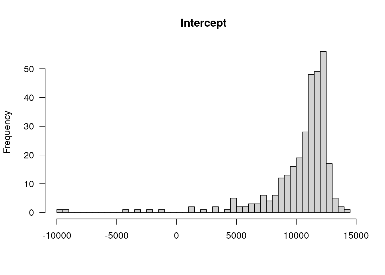

Past versions of “Process phenotype on the genotyped animals-7.png”

Version	Author	Date
2470aab	xhyuo	2022-12-24

plotPheno(WT144, pheno.col=13, xlab = "")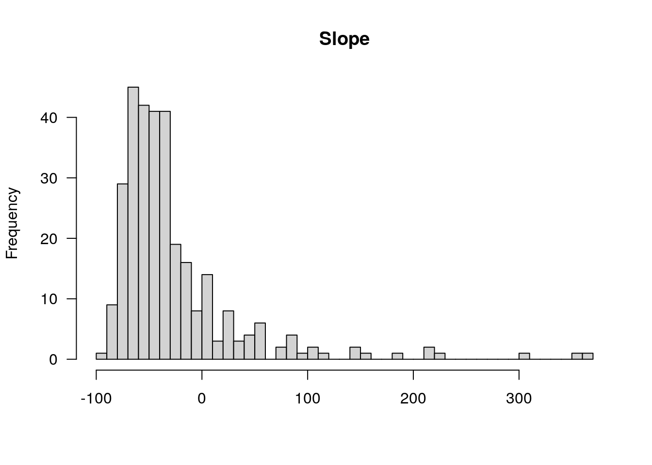

Past versions of “Process phenotype on the genotyped animals-8.png”

Version	Author	Date
2470aab	xhyuo	2022-12-24

Run qtl

#run qtl
print(summary(WT144))

    F2 intercross

    No. individuals:    309 

    No. phenotypes:     13 
    Percent phenotyped: 100 100 100 99.7 100 100 99.7 90.9 100 99.7 90.9 100 100 

    No. chromosomes:    18 
        Autosomes:      1 2 3 4 5 7 8 9 10 11 12 13 14 15 16 17 18 19 

    Total markers:      78 
    No. markers:        5 8 7 1 22 4 3 5 1 1 4 2 4 2 2 2 2 3 
    Percent genotyped:  98 
    Genotypes (%):      AA:25.9  AB:50.7  BB:23.3  not BB:0.0  not AA:0.0 

WT144 <- drop.nullmarkers(WT144)
covars <- model.matrix(~ Gender, WT144$pheno)[,-1]
#idx 
idx <- c(11, 13)
out.mr <- operm <- st <- list()
#loop for each pheno
for (i in 1:length(idx)){
  out.mr[[i]] <- scanone(WT144, pheno.col=idx[[i]], method="mr", addcovar=covars)
  out.mr[[i]]$lod[is.infinite(out.mr[[i]]$lod)]=0
  print(summary(out.mr[[i]]))
  #operm
  operm[[i]] <-scanone(WT144, pheno.col=idx[[i]], n.perm=1000, method="mr", addcovar=covars)
  print(summary(operm[[i]]))
  #scantwo
  st[[i]] <- scantwo(WT144, pheno.col = idx[[i]], method="mr")
}

Warning in checkcovar(cross, pheno.col, addcovar, intcovar, perm.strata, : Dropping 28 individuals with missing phenotypes.

                      chr  pos     lod
chr1-188155143-.-G-A    1 92.2  1.1232
chr2-137498061-.-T-A    2 67.9  1.8838
chr3-98881230-.-G-A     3 42.9  1.1117
chr4-32821418-.-C-T     4 14.4  0.8050
chr5-136844385-.-T-G    5 76.1 26.1801
chr7-35061547-.-A-G     7 20.9  0.4206
chr8-112465004-.-G-A    8 58.6  0.1365
chr9-64698947-.-C-T     9 34.9  0.2296
chr10-24134777-.-A-T   10 11.5  2.0508
chr11-96730656-.-A-G   11 60.1  0.0908
chr12-43136399-.-A-T   12 19.5  0.9613
chr13-115031098-.-T-C  13 64.6  2.2455
chr14-69691477-.-G-T   14 36.1  6.0905
chr15-58605950-.-C-G   15 25.0  0.0869
chr16-32593683-.-A-G   16 23.0  0.2049
chr17-69219676-.-G-A   17 40.3  0.7094
chr18-51300216-.-T-A   18 27.9  0.1625
chr19-45958839-.-A-T   19 38.8  0.7538

Warning in checkcovar(cross, pheno.col, addcovar, intcovar, perm.strata, : Dropping 28 individuals with missing phenotypes.

Permutation 20 
Permutation 40 
Permutation 60 
Permutation 80 
Permutation 100 
Permutation 120 
Permutation 140 
Permutation 160 
Permutation 180 
Permutation 200 
Permutation 220 
Permutation 240 
Permutation 260 
Permutation 280 
Permutation 300 
Permutation 320 
Permutation 340 
Permutation 360 
Permutation 380 
Permutation 400 
Permutation 420 
Permutation 440 
Permutation 460 
Permutation 480 
Permutation 500 
Permutation 520 
Permutation 540 
Permutation 560 
Permutation 580 
Permutation 600 
Permutation 620 
Permutation 640 
Permutation 660 
Permutation 680 
Permutation 700 
Permutation 720 
Permutation 740 
Permutation 760 
Permutation 780 
Permutation 800 
Permutation 820 
Permutation 840 
Permutation 860 
Permutation 880 
Permutation 900 
Permutation 920 
Permutation 940 
Permutation 960 
Permutation 980 
Permutation 1000 
LOD thresholds (1000 permutations)
     lod
5%  3.10
10% 2.68

Warning in checkcovar(cross, pheno.col, addcovar, intcovar, perm.strata, : Dropping 28 individuals with missing phenotypes.

 --Running scanone
 --Running scantwo
 (1,1)
 (1,2)
 (1,3)
 (1,4)
 (1,5)
 (1,7)
 (1,8)
 (1,9)
 (1,10)
 (1,11)
 (1,12)
 (1,13)
 (1,14)
 (1,15)
 (1,16)
 (1,17)
 (1,18)
 (1,19)
 (2,2)
 (2,3)
 (2,4)
 (2,5)
 (2,7)
 (2,8)
 (2,9)
 (2,10)
 (2,11)
 (2,12)
 (2,13)
 (2,14)
 (2,15)
 (2,16)
 (2,17)
 (2,18)
 (2,19)
 (3,3)
 (3,4)
 (3,5)
 (3,7)
 (3,8)
 (3,9)
 (3,10)
 (3,11)
 (3,12)
 (3,13)
 (3,14)
 (3,15)
 (3,16)
 (3,17)
 (3,18)
 (3,19)
 (4,4)
 (4,5)
 (4,7)
 (4,8)
 (4,9)
 (4,10)
 (4,11)
 (4,12)
 (4,13)
 (4,14)
 (4,15)
 (4,16)
 (4,17)
 (4,18)
 (4,19)
 (5,5)
 (5,7)
 (5,8)
 (5,9)
 (5,10)
 (5,11)
 (5,12)
 (5,13)
 (5,14)
 (5,15)
 (5,16)
 (5,17)
 (5,18)
 (5,19)
 (7,7)
 (7,8)
 (7,9)
 (7,10)
 (7,11)
 (7,12)
 (7,13)
 (7,14)
 (7,15)
 (7,16)
 (7,17)
 (7,18)
 (7,19)
 (8,8)
 (8,9)
 (8,10)
 (8,11)
 (8,12)
 (8,13)
 (8,14)
 (8,15)
 (8,16)
 (8,17)
 (8,18)
 (8,19)
 (9,9)
 (9,10)
 (9,11)
 (9,12)
 (9,13)
 (9,14)
 (9,15)
 (9,16)
 (9,17)
 (9,18)
 (9,19)
 (10,10)
 (10,11)
 (10,12)
 (10,13)
 (10,14)
 (10,15)
 (10,16)
 (10,17)
 (10,18)
 (10,19)
 (11,11)
 (11,12)
 (11,13)
 (11,14)
 (11,15)
 (11,16)
 (11,17)
 (11,18)
 (11,19)
 (12,12)
 (12,13)
 (12,14)
 (12,15)
 (12,16)
 (12,17)
 (12,18)
 (12,19)
 (13,13)
 (13,14)
 (13,15)
 (13,16)
 (13,17)
 (13,18)
 (13,19)
 (14,14)
 (14,15)
 (14,16)
 (14,17)
 (14,18)
 (14,19)
 (15,15)
 (15,16)
 (15,17)
 (15,18)
 (15,19)
 (16,16)
 (16,17)
 (16,18)
 (16,19)
 (17,17)
 (17,18)
 (17,19)
 (18,18)
 (18,19)
 (19,19)
                      chr  pos     lod
chr1-65643621-.-C-A     1 33.3  1.4142
chr2-137498061-.-T-A    2 67.9  2.3977
chr3-59218564-.-T-A     3 29.0  1.5114
chr4-32821418-.-C-T     4 14.4  0.9584
chr5-136332619-.-C-A    5 76.0 28.2723
chr7-35061547-.-A-G     7 20.9  0.2899
chr8-112465004-.-G-A    8 58.6  0.2728
chr9-69415567-.-T-A     9 38.6  0.5506
chr10-24134777-.-A-T   10 11.5  2.1472
chr11-96730656-.-A-G   11 60.1  0.2845
chr12-43136399-.-A-T   12 19.5  1.1682
chr13-115031098-.-T-C  13 64.6  2.0179
chr14-69691477-.-G-T   14 36.1  6.3651
chr15-58605950-.-C-G   15 25.0  0.2664
chr16-32593683-.-A-G   16 23.0  0.4304
chr17-69219676-.-G-A   17 40.3  0.9353
chr18-89347666-.-A-G   18 59.0  0.0746
chr19-45958839-.-A-T   19 38.8  0.5790
Permutation 20 
Permutation 40 
Permutation 60 
Permutation 80 
Permutation 100 
Permutation 120 
Permutation 140 
Permutation 160 
Permutation 180 
Permutation 200 
Permutation 220 
Permutation 240 
Permutation 260 
Permutation 280 
Permutation 300 
Permutation 320 
Permutation 340 
Permutation 360 
Permutation 380 
Permutation 400 
Permutation 420 
Permutation 440 
Permutation 460 
Permutation 480 
Permutation 500 
Permutation 520 
Permutation 540 
Permutation 560 
Permutation 580 
Permutation 600 
Permutation 620 
Permutation 640 
Permutation 660 
Permutation 680 
Permutation 700 
Permutation 720 
Permutation 740 
Permutation 760 
Permutation 780 
Permutation 800 
Permutation 820 
Permutation 840 
Permutation 860 
Permutation 880 
Permutation 900 
Permutation 920 
Permutation 940 
Permutation 960 
Permutation 980 
Permutation 1000 
LOD thresholds (1000 permutations)
     lod
5%  3.10
10% 2.75
 --Running scanone
 --Running scantwo
 (1,1)
 (1,2)
 (1,3)
 (1,4)
 (1,5)
 (1,7)
 (1,8)
 (1,9)
 (1,10)
 (1,11)
 (1,12)
 (1,13)
 (1,14)
 (1,15)
 (1,16)
 (1,17)
 (1,18)
 (1,19)
 (2,2)
 (2,3)
 (2,4)
 (2,5)
 (2,7)
 (2,8)
 (2,9)
 (2,10)
 (2,11)
 (2,12)
 (2,13)
 (2,14)
 (2,15)
 (2,16)
 (2,17)
 (2,18)
 (2,19)
 (3,3)
 (3,4)
 (3,5)
 (3,7)
 (3,8)
 (3,9)
 (3,10)
 (3,11)
 (3,12)
 (3,13)
 (3,14)
 (3,15)
 (3,16)
 (3,17)
 (3,18)
 (3,19)
 (4,4)
 (4,5)
 (4,7)
 (4,8)
 (4,9)
 (4,10)
 (4,11)
 (4,12)
 (4,13)
 (4,14)
 (4,15)
 (4,16)
 (4,17)
 (4,18)
 (4,19)
 (5,5)
 (5,7)
 (5,8)
 (5,9)
 (5,10)
 (5,11)
 (5,12)
 (5,13)
 (5,14)
 (5,15)
 (5,16)
 (5,17)
 (5,18)
 (5,19)
 (7,7)
 (7,8)
 (7,9)
 (7,10)
 (7,11)
 (7,12)
 (7,13)
 (7,14)
 (7,15)
 (7,16)
 (7,17)
 (7,18)
 (7,19)
 (8,8)
 (8,9)
 (8,10)
 (8,11)
 (8,12)
 (8,13)
 (8,14)
 (8,15)
 (8,16)
 (8,17)
 (8,18)
 (8,19)
 (9,9)
 (9,10)
 (9,11)
 (9,12)
 (9,13)
 (9,14)
 (9,15)
 (9,16)
 (9,17)
 (9,18)
 (9,19)
 (10,10)
 (10,11)
 (10,12)
 (10,13)
 (10,14)
 (10,15)
 (10,16)
 (10,17)
 (10,18)
 (10,19)
 (11,11)
 (11,12)
 (11,13)
 (11,14)
 (11,15)
 (11,16)
 (11,17)
 (11,18)
 (11,19)
 (12,12)
 (12,13)
 (12,14)
 (12,15)
 (12,16)
 (12,17)
 (12,18)
 (12,19)
 (13,13)
 (13,14)
 (13,15)
 (13,16)
 (13,17)
 (13,18)
 (13,19)
 (14,14)
 (14,15)
 (14,16)
 (14,17)
 (14,18)
 (14,19)
 (15,15)
 (15,16)
 (15,17)
 (15,18)
 (15,19)
 (16,16)
 (16,17)
 (16,18)
 (16,19)
 (17,17)
 (17,18)
 (17,19)
 (18,18)
 (18,19)
 (19,19)

save(out.mr, operm, st, file = "output/qtl.out.obj.mixedmodel.final.RData")

Plot on run qtl

name = "WT144_plot"
#print
print(summary(WT144))

    F2 intercross

    No. individuals:    309 

    No. phenotypes:     13 
    Percent phenotyped: 100 100 100 99.7 100 100 99.7 90.9 100 99.7 90.9 100 100 

    No. chromosomes:    18 
        Autosomes:      1 2 3 4 5 7 8 9 10 11 12 13 14 15 16 17 18 19 

    Total markers:      78 
    No. markers:        5 8 7 1 22 4 3 5 1 1 4 2 4 2 2 2 2 3 
    Percent genotyped:  98 
    Genotypes (%):      AA:25.9  AB:50.7  BB:23.3  not BB:0.0  not AA:0.0 

WT144 <- drop.nullmarkers(WT144)
covars <- model.matrix(~ Gender, WT144$pheno)[,-1]
#idx 
idx <- c(11, 13)
#map
map <- purrr::map(WT144$geno, ~(.x$map))
attr(map, "is_x_chr") <- structure(c(rep(FALSE,18)), names=c(1:5, 7:19))

load("output/qtl.out.obj.mixedmodel.final.RData")
#loop for each pheno
for (i in 1:length(idx)){
  print(colnames(WT144$pheno)[idx[[i]]])
  #operm_hist
  #pdf(paste0("output/", name,"-", colnames(WT144$pheno)[idx[[i]]], ".pdf"), width = 10, height = 10)
  plot(operm[[i]][!is.infinite(operm[[i]])], main=paste(name, colnames(WT144$pheno)[idx[[i]]], sep="-"))
  #mrscan_pheno
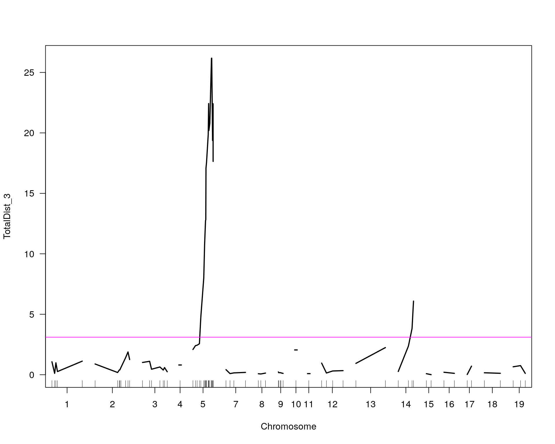
  plot(out.mr[[i]], ylab=colnames(WT144$pheno)[idx[[i]]])
  add.threshold(out.mr[[i]], perms = operm[[i]], alpha = 0.05, col="magenta")
  #pxg
  peak = summary(out.mr[[i]], threshold=summary(operm[[i]], alpha = 0.05)[[1]])
  print(peak)
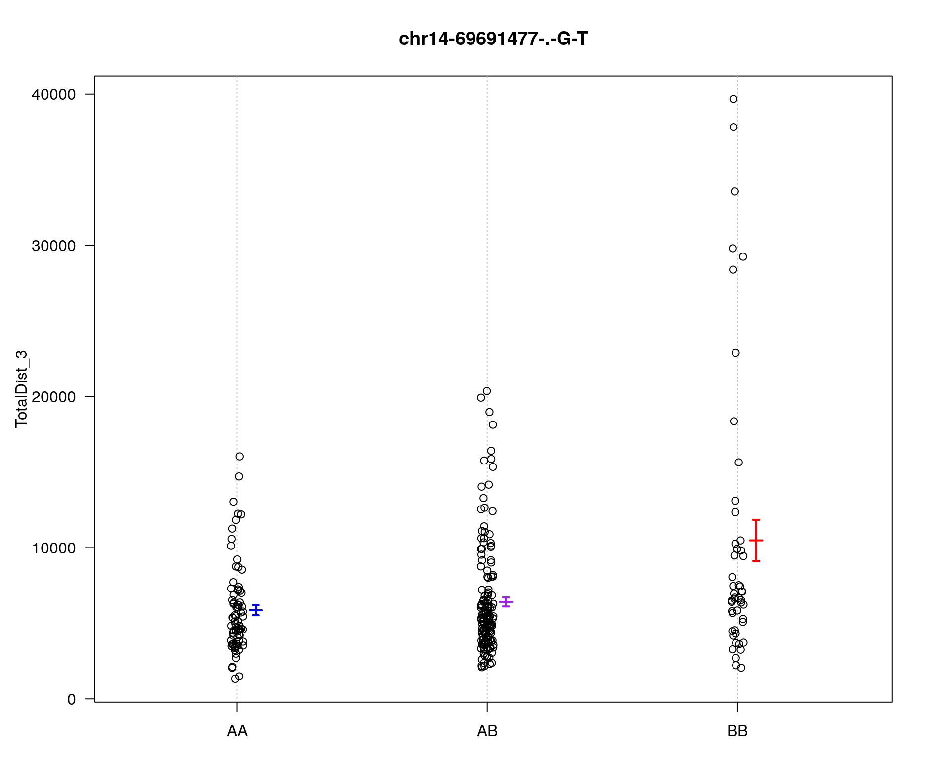
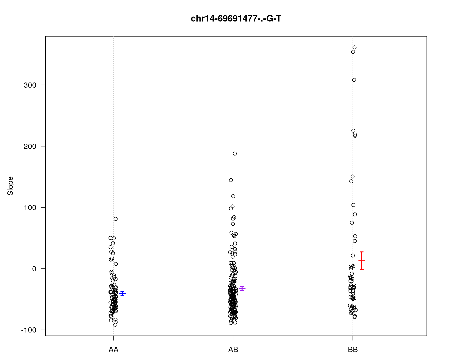
  marker = c("chr5-136332619-.-C-A", "chr14-69691477-.-G-T")
  for (mar in marker){
    par(mar=c(3, 5, 4, 3))
    plotPXG(WT144, marker=mar, jitter = 0.25, pheno.col = idx[[i]], infer=F, main=paste(mar),
            mgp=c(3.4,1,0))
  }
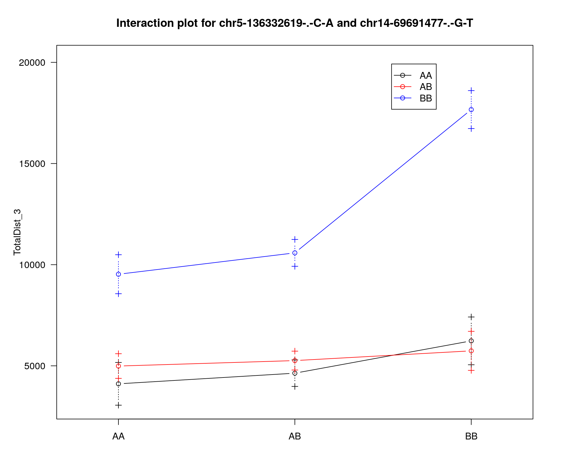
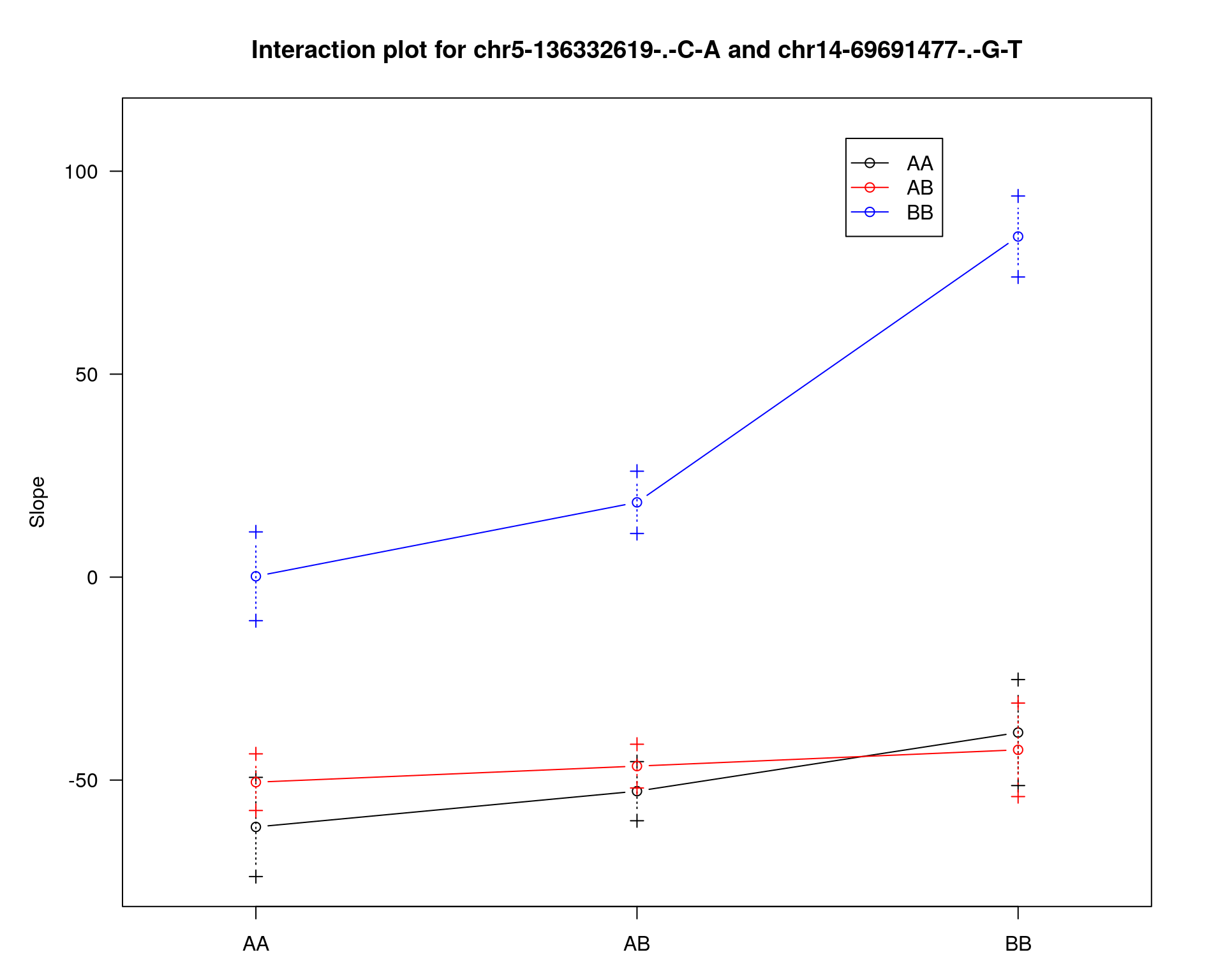
  #interaction_effect
  effectplot(WT144, 
             mname1 = marker[[1]], 
             mname2 = marker[[2]], 
             pheno.col = idx[[i]], add.legend=T, legend.lab = "")
  
    ##Multiple-QTL analyses 
  # After performing the single- and two-QTL genome scans, it’s best to bring the identified loci together into a joint model, which we then refine and from which we may explore the possibility of further QTL. In this effort, we work with “QTL objects” created by makeqtl(). We fit multiple-QTL models with fitqtl(). A number of additional functions will be introduced below.
  #First, we create a QTL object containing the loci on chr 5 and 14. 
  #chr5-136332619-.-C-A  75.97770
  #chr14-69691477-.-G-T  36.07219
  WT144 <- sim.geno(WT144, n.draws=64)
  qtl <- makeqtl(WT144, chr=c(5,14), pos=c(75.97770, 36.07219), what="draws")
  out.fq <- fitqtl(WT144, pheno.col=idx[[i]], qtl=qtl) 
  print(summary(out.fq))
  #We may obtain the estimated effects of the QTL via get.ests=TRUE. We use dropone=FALSE to suppress the drop-one-term analysis.
  print(summary(fitqtl(WT144, pheno.col=idx[[i]], qtl=qtl, get.ests=TRUE, dropone=FALSE)))
  #To assess the possibility of an interaction between the two QTL, we may fit the model with the interaction, indicated via a model “formula”.
  print("To assess the possibility of an interaction between the two QTL")
  out.fqi <- fitqtl(WT144, pheno.col=idx[[i]], qtl=qtl, formula=y~Q1+Q2+Q1:Q2) 
  print(summary(out.fqi))
  
  #complete_scan2
  plot(st[[i]])
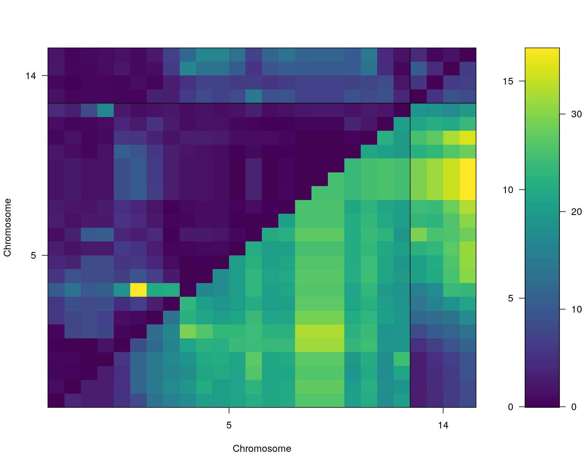
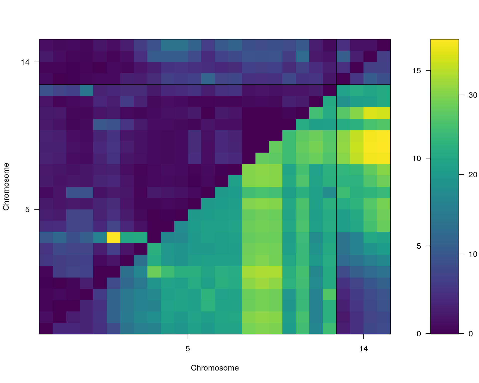
  #toptwo_scan2
  plot(st[[i]], chr = summary(out.mr[[i]])[order(-summary(out.mr[[i]])$lod), "chr"][1:2])
  #dev.off()
}

[1] "TotalDist_3"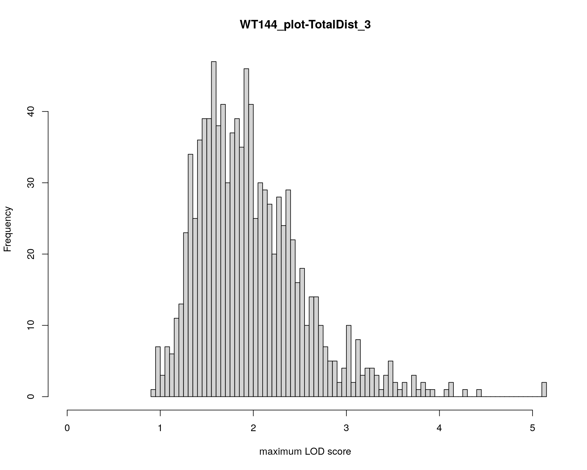

Past versions of “Plot on run qtl-1.png”

Version	Author	Date
2470aab	xhyuo	2022-12-24

Past versions of “Plot on run qtl-2.png”

Version	Author	Date
2470aab	xhyuo	2022-12-24

                     chr  pos   lod
chr5-136332619-.-C-A   5 76.0 26.18
chr14-69691477-.-G-T  14 36.1  6.09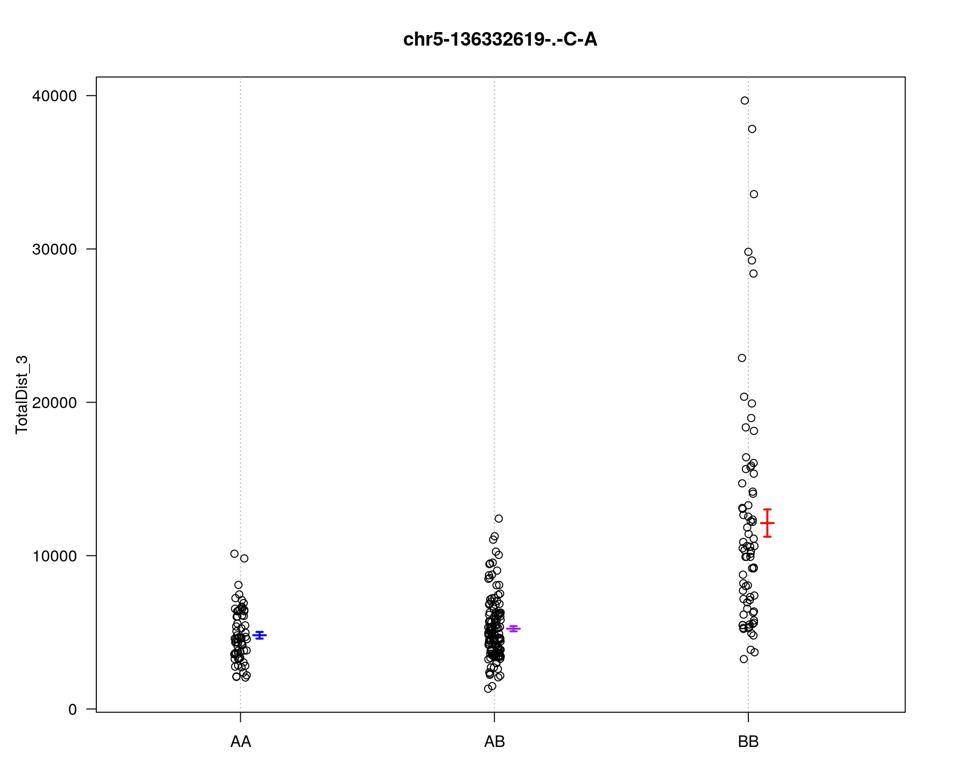

Past versions of “Plot on run qtl-3.png”

Version	Author	Date
2470aab	xhyuo	2022-12-24

Past versions of “Plot on run qtl-4.png”

Version	Author	Date
2470aab	xhyuo	2022-12-24

Past versions of “Plot on run qtl-5.png”

Version	Author	Date
2470aab	xhyuo	2022-12-24

        fitqtl summary

Method: multiple imputation 
Model:  normal phenotype
Number of observations : 281 

Full model result
----------------------------------  
Model formula: y ~ Q1 + Q2 

       df         SS        MS      LOD     %var Pvalue(Chi2) Pvalue(F)
Model   4 3170953192 792738298 31.45606 40.28087            0         0
Error 276 4701152932  17033163                                         
Total 280 7872106124                                                   


Drop one QTL at a time ANOVA table: 
----------------------------------  
        df Type III SS    LOD   %var F value Pvalue(Chi2) Pvalue(F)    
5@76.0   2   2.423e+09 25.367 30.783   71.13            0   < 2e-16 ***
14@36.1  2   4.478e+08  5.552  5.688   13.14            0  3.52e-06 ***
---
Signif. codes:  0 '***' 0.001 '**' 0.01 '*' 0.05 '.' 0.1 ' ' 1


        fitqtl summary

Method: multiple imputation 
Model:  normal phenotype
Number of observations : 281 

Full model result
----------------------------------  
Model formula: y ~ Q1 + Q2 

       df         SS        MS      LOD     %var Pvalue(Chi2) Pvalue(F)
Model   4 3170953192 792738298 31.45606 40.28087            0         0
Error 276 4701152932  17033163                                         
Total 280 7872106124                                                   


Estimated effects:
-----------------
              est      SE      t
Intercept  7106.1   251.6 28.248
5@76.0a    3549.0   349.2 10.162
5@76.0d   -2908.4   497.5 -5.846
14@36.1a   1818.7   380.1  4.785
14@36.1d  -1335.8   503.4 -2.654

[1] "To assess the possibility of an interaction between the two QTL"

        fitqtl summary

Method: multiple imputation 
Model:  normal phenotype
Number of observations : 281 

Full model result
----------------------------------  
Model formula: y ~ Q1 + Q2 + Q1:Q2 

       df         SS        MS      LOD     %var Pvalue(Chi2) Pvalue(F)
Model   8 3558421585 444802698 36.70458 45.20292            0         0
Error 272 4313684539  15859134                                         
Total 280 7872106124                                                   


Drop one QTL at a time ANOVA table: 
----------------------------------  
               df Type III SS    LOD   %var F value Pvalue(Chi2) Pvalue(F)    
5@76.0          6   2.811e+09 30.615 35.705  29.539            0   < 2e-16 ***
14@36.1         6   8.353e+08 10.800 10.610   8.778            0  9.42e-09 ***
5@76.0:14@36.1  4   3.875e+08  5.249  4.922   6.108            0  0.000101 ***
---
Signif. codes:  0 '***' 0.001 '**' 0.01 '*' 0.05 '.' 0.1 ' ' 1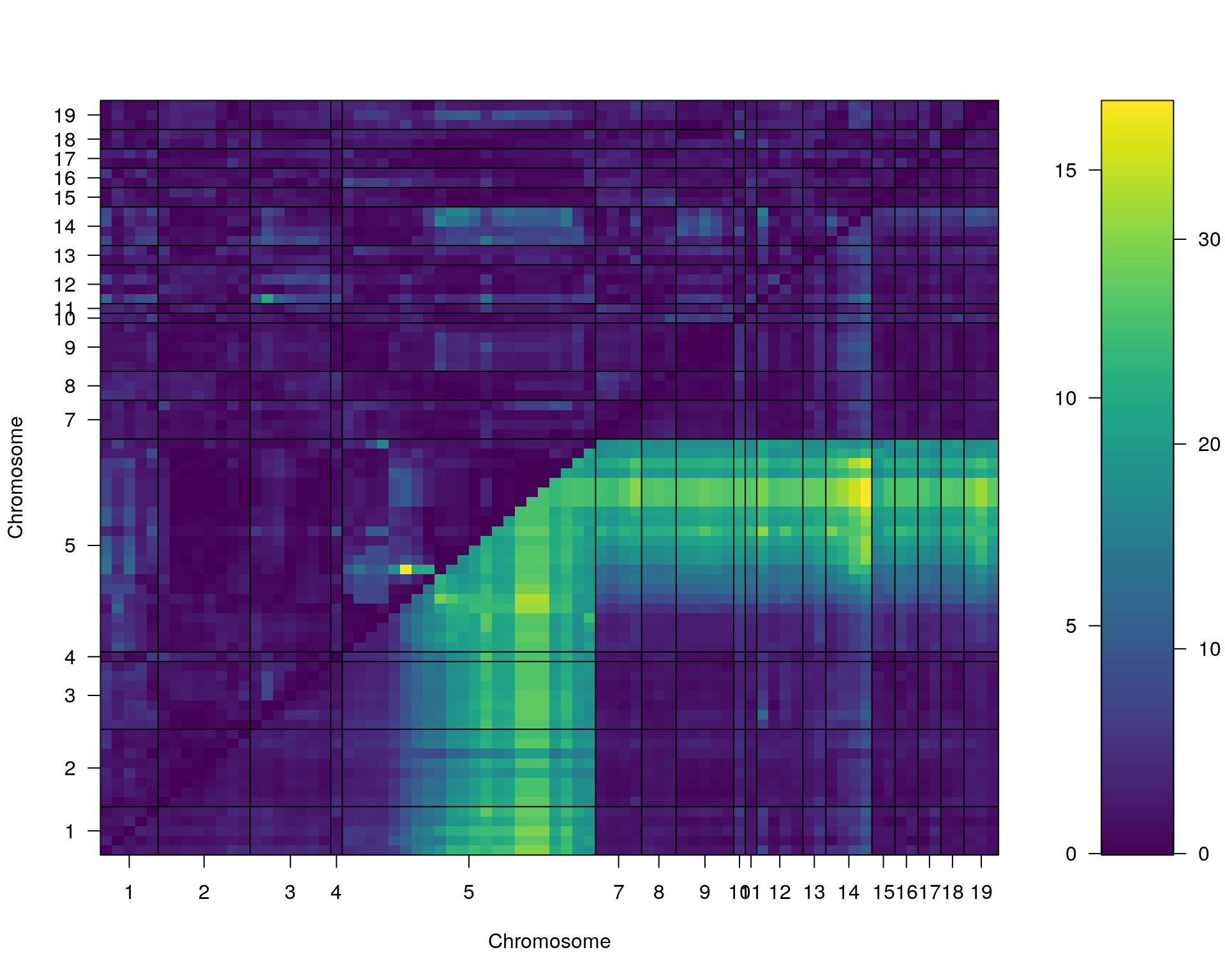

Past versions of “Plot on run qtl-6.png”

Version	Author	Date
2470aab	xhyuo	2022-12-24

Past versions of “Plot on run qtl-7.png”

Version	Author	Date
2470aab	xhyuo	2022-12-24

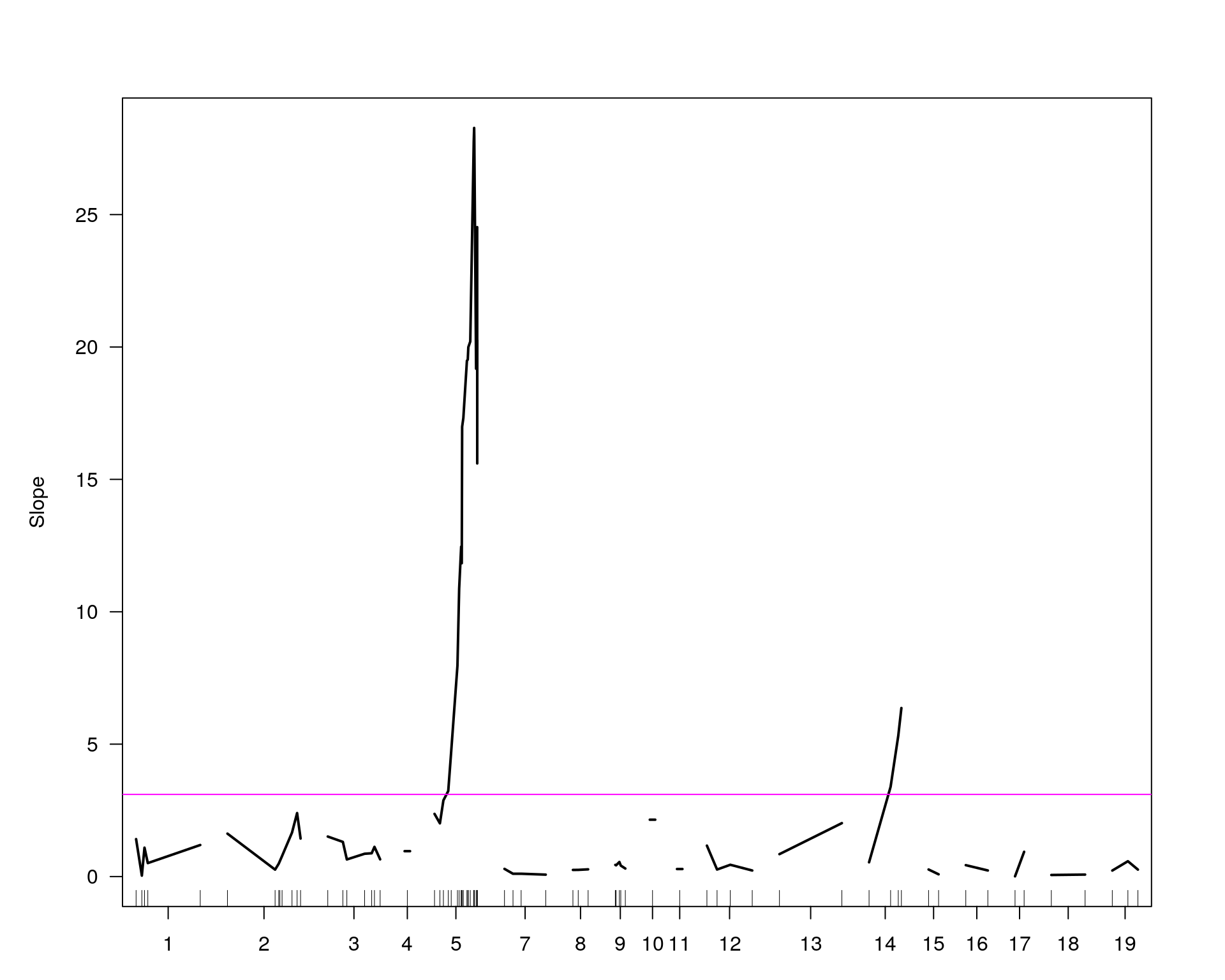
[1] "Slope"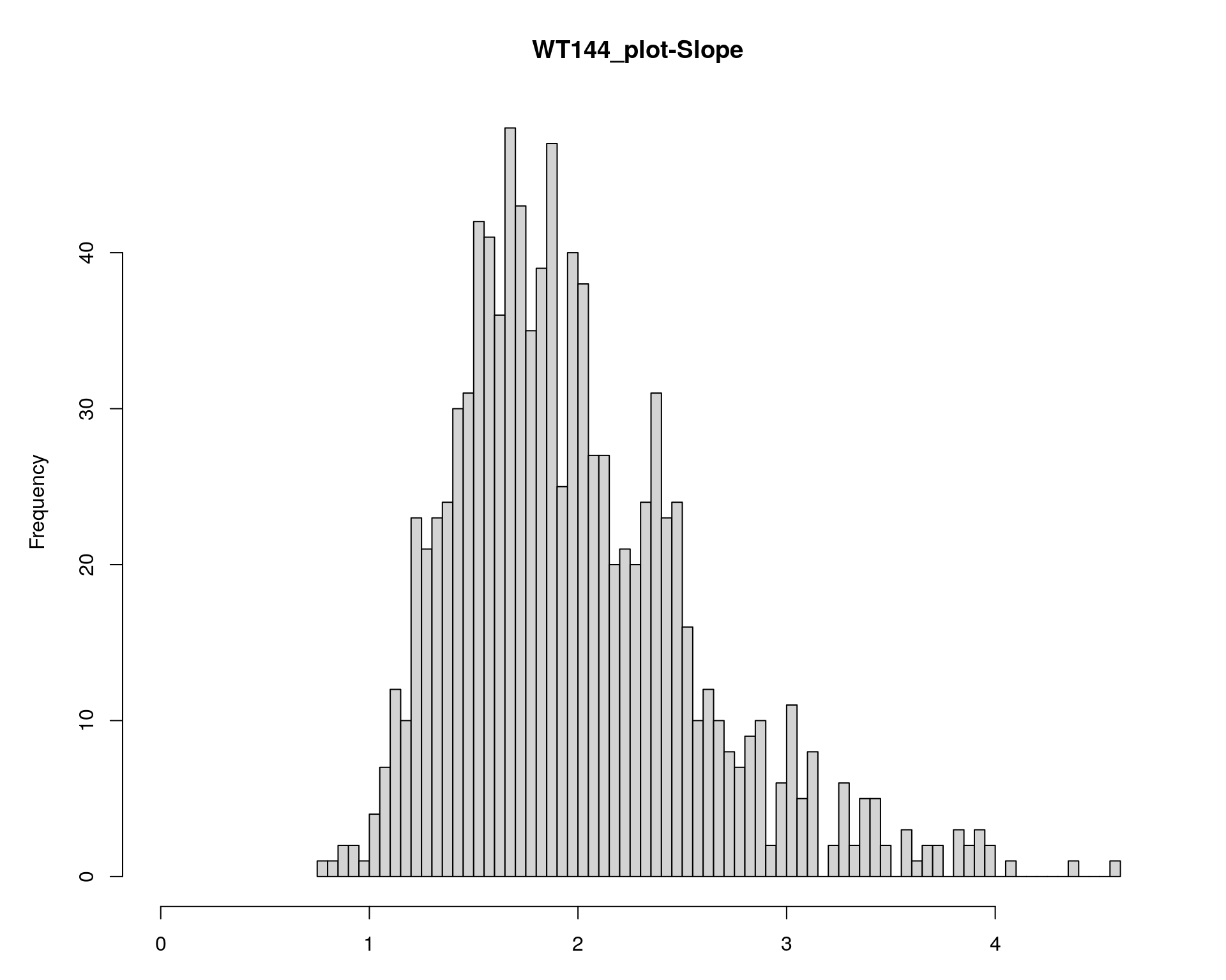

Past versions of “Plot on run qtl-8.png”

Version	Author	Date
2470aab	xhyuo	2022-12-24

Past versions of “Plot on run qtl-9.png”

Version	Author	Date
2470aab	xhyuo	2022-12-24

                     chr  pos   lod
chr5-136332619-.-C-A   5 76.0 28.27
chr14-69691477-.-G-T  14 36.1  6.37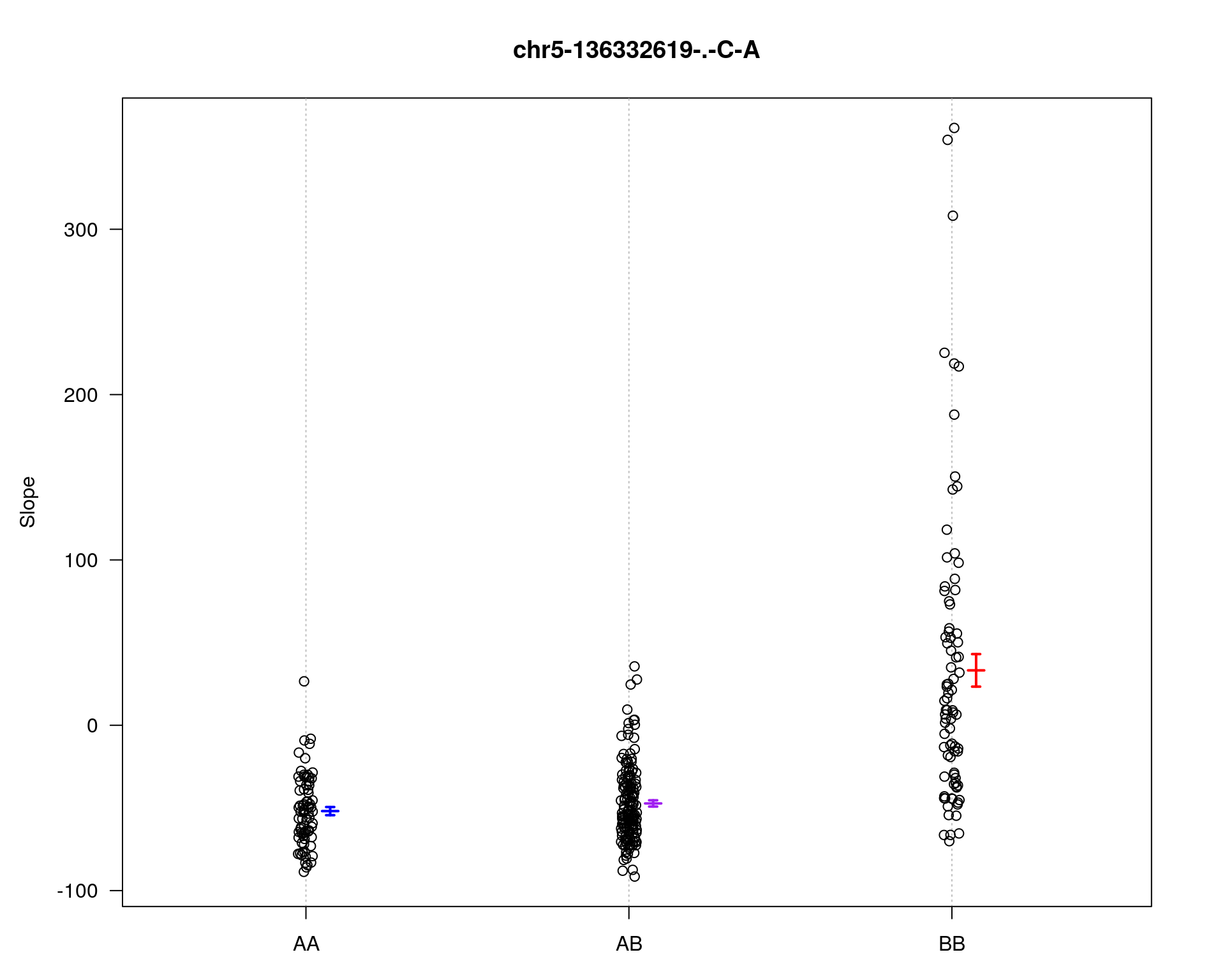

Past versions of “Plot on run qtl-10.png”

Version	Author	Date
2470aab	xhyuo	2022-12-24

Past versions of “Plot on run qtl-11.png”

Version	Author	Date
2470aab	xhyuo	2022-12-24

Past versions of “Plot on run qtl-12.png”

Version	Author	Date
2470aab	xhyuo	2022-12-24

        fitqtl summary

Method: multiple imputation 
Model:  normal phenotype
Number of observations : 309 

Full model result
----------------------------------  
Model formula: y ~ Q1 + Q2 

       df        SS         MS      LOD    %var Pvalue(Chi2) Pvalue(F)
Model   4  464953.1 116238.280 32.79348 38.6599            0         0
Error 304  737722.4   2426.718                                        
Total 308 1202675.5                                                   


Drop one QTL at a time ANOVA table: 
----------------------------------  
        df Type III SS    LOD   %var F value Pvalue(Chi2) Pvalue(F)    
5@76.0   2      355772 26.408 29.582   73.30            0   < 2e-16 ***
14@36.1  2       55117  4.835  4.583   11.36            0  1.75e-05 ***
---
Signif. codes:  0 '***' 0.001 '**' 0.01 '*' 0.05 '.' 0.1 ' ' 1


        fitqtl summary

Method: multiple imputation 
Model:  normal phenotype
Number of observations : 309 

Full model result
----------------------------------  
Model formula: y ~ Q1 + Q2 

       df        SS         MS      LOD    %var Pvalue(Chi2) Pvalue(F)
Model   4  464953.1 116238.280 32.79348 38.6599            0         0
Error 304  737722.4   2426.718                                        
Total 308 1202675.5                                                   


Estimated effects:
-----------------
              est      SE      t
Intercept -26.034   2.858 -9.109
5@76.0a    40.855   3.927 10.405
5@76.0d   -33.307   5.693 -5.850
14@36.1a   19.763   4.307  4.589
14@36.1d  -11.513   5.726 -2.011

[1] "To assess the possibility of an interaction between the two QTL"

        fitqtl summary

Method: multiple imputation 
Model:  normal phenotype
Number of observations : 309 

Full model result
----------------------------------  
Model formula: y ~ Q1 + Q2 + Q1:Q2 

       df        SS        MS      LOD     %var Pvalue(Chi2) Pvalue(F)
Model   8  507503.1 63437.888 36.77964 42.19784            0         0
Error 300  695172.4  2317.241                                         
Total 308 1202675.5                                                   


Drop one QTL at a time ANOVA table: 
----------------------------------  
               df Type III SS    LOD   %var F value Pvalue(Chi2) Pvalue(F)    
5@76.0          6      398322 30.394 33.120  28.649        0.000   < 2e-16 ***
14@36.1         6       97667  8.821  8.121   7.025        0.000  5.22e-07 ***
5@76.0:14@36.1  4       42550  3.986  3.538   4.591        0.001    0.0013 ** 
---
Signif. codes:  0 '***' 0.001 '**' 0.01 '*' 0.05 '.' 0.1 ' ' 1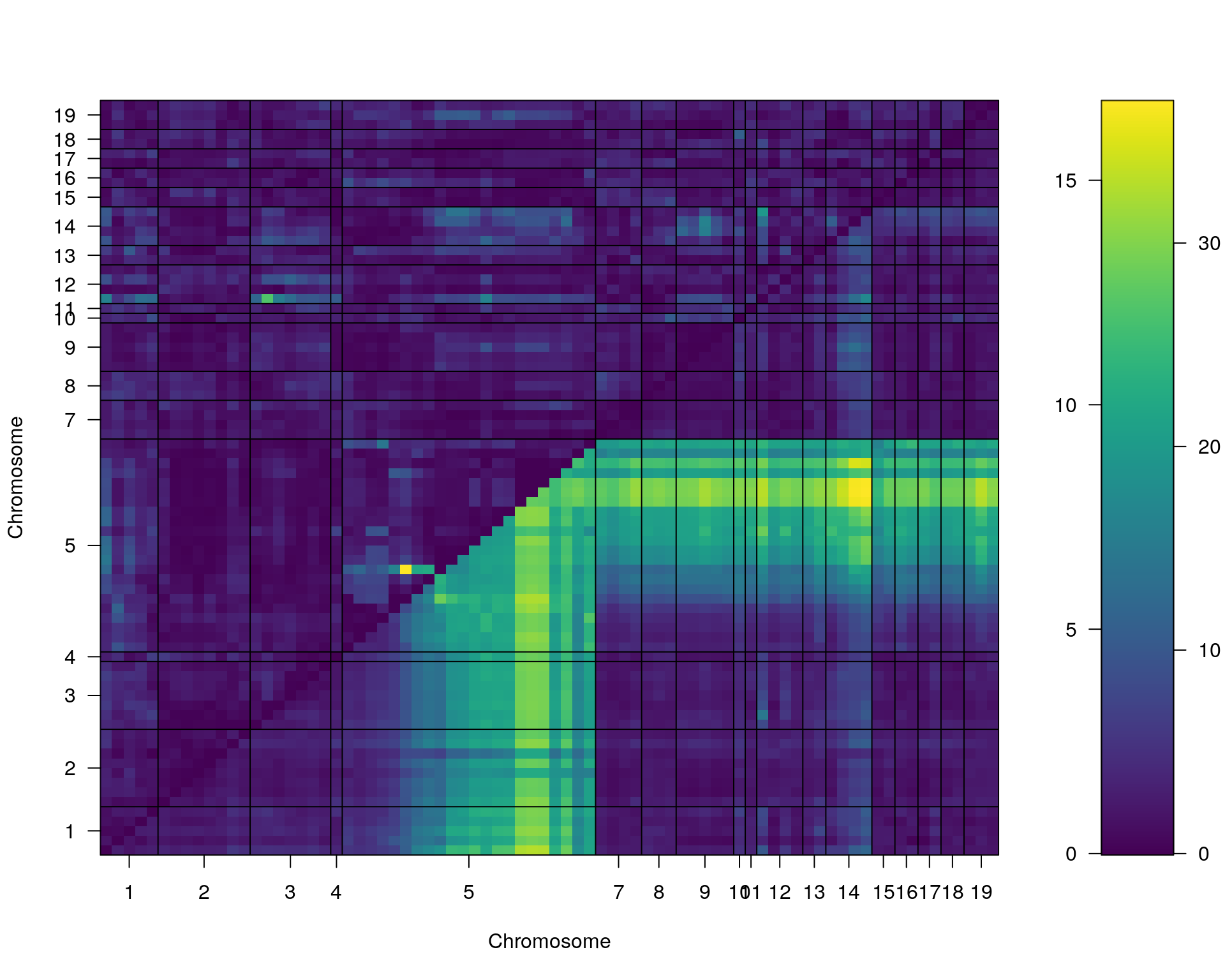

Past versions of “Plot on run qtl-13.png”

Version	Author	Date
2470aab	xhyuo	2022-12-24

Past versions of “Plot on run qtl-14.png”

Version	Author	Date
2470aab	xhyuo	2022-12-24

#plot phenotypes: slope and totaldistance3
plot(out.mr[[2]], col= "blue", ylim = c(0, 30), ylab = "LOD score")
plot(out.mr[[1]], col= "green", add=TRUE)
abline(h=3.2, col="red", lty=2, lwd=3)
# Add a legend
legend("topright", 
       legend=c("Slope", "Total distance traveled"),
       col=c("blue", "green"), lty=1, cex=0.8)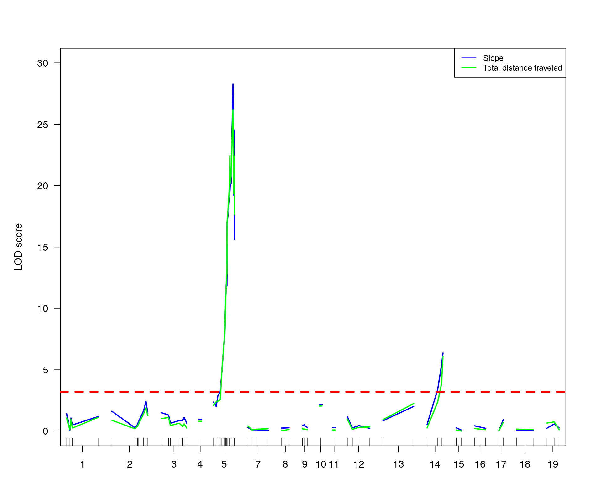

Past versions of “Plot on run qtl-15.png”

Version	Author	Date
2470aab	xhyuo	2022-12-24

#only at chr 5 and 14
#plot phenotypes: slope and totaldistance3
plot(out.mr[[2]], col= "blue", ylim = c(0, 30), ylab = "LOD score", chr = c(5, 14))
plot(out.mr[[1]], col= "green", add=TRUE, chr = c(5, 14))
abline(h=3.2, col="red", lty=2, lwd=3)
# Add a legend
legend("topright", 
       legend=c("Slope", "Total distance traveled"),
       col=c("blue", "green"), lty=1, cex=0.8)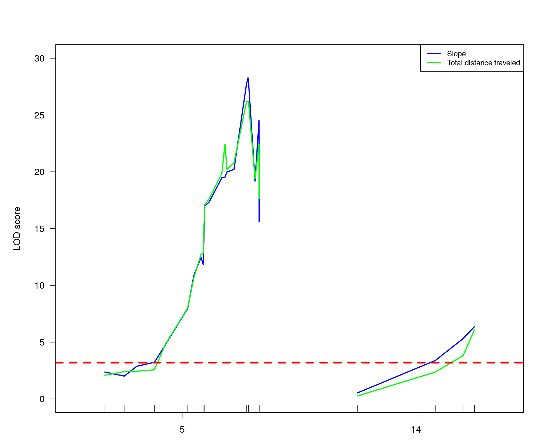

Past versions of “Plot on run qtl-16.png”

Version	Author	Date
2470aab	xhyuo	2022-12-24

#Interval estimates of the location of QTL are commonly obtained via 1.5-LOD support intervals,
lodint.chr5.slope = lodint(out.mr[[2]], chr= 5)
lodint.chr5.slope

                     chr      pos      lod
chr5-133052642-.-T-G   5 72.40547 20.20584
chr5-136332619-.-C-A   5 75.97770 28.27231
chr5-138956439-.-T-C   5 77.76853 19.17899

lodint.chr14.slope = lodint(out.mr[[2]], chr= 14)
lodint.chr14.slope

                      chr      pos      lod
chr14-50642778-.-G-A   14 26.14972 3.390345
chr14-69691477-.-G-T   14 36.07219 6.365103
chr14-69691477-.-G-T   14 36.07219 6.365103

lodint.chr5.TotalDist3 = lodint(out.mr[[1]], chr= 5)
lodint.chr5.TotalDist3

                     chr      pos      lod
chr5-133052642-.-T-G   5 72.40547 20.78647
chr5-136332619-.-C-A   5 75.97770 26.18011
chr5-136844385-.-T-G   5 76.10078 26.18011
chr5-138956439-.-T-C   5 77.76853 19.37148

lodint.chr14.TotalDist3 = lodint(out.mr[[1]], chr= 14)
lodint.chr14.TotalDist3

                      chr      pos      lod
chr14-62407765-.-T-A   14 33.20623 3.823005
chr14-69691477-.-G-T   14 36.07219 6.090514
chr14-69691477-.-G-T   14 36.07219 6.090514

#loop for each pheno
for (i in 1:length(idx)){  
  print(colnames(WT144$pheno)[idx[[i]]])
  #save plots
  #operm_hist
  pdf(paste0("output/", name,"-", colnames(WT144$pheno)[idx[[i]]], ".pdf"), width = 10, height = 10)
  plot(operm[[i]][!is.infinite(operm[[i]])], main=paste(name, colnames(WT144$pheno)[idx[[i]]], sep="-"))
  #mrscan_pheno
  plot(out.mr[[i]], ylab=colnames(WT144$pheno)[idx[[i]]])
  add.threshold(out.mr[[i]], perms = operm[[i]], alpha = 0.05, col="magenta")
  #pxg
  peak = summary(out.mr[[i]], threshold=summary(operm[[i]], alpha = 0.05)[[1]])
  print(peak)
  marker = c("chr5-136332619-.-C-A", "chr14-69691477-.-G-T")
  for (mar in marker){
    par(mar=c(3, 5, 4, 3))
    plotPXG(WT144, marker=mar, jitter = 0.25, pheno.col = idx[[i]], infer=F, main=paste(mar),
            mgp=c(3.4,1,0))
  }
  #interaction_effect
  effectplot(WT144, 
             mname1 = rownames(peak)[1], 
             mname2 = rownames(peak)[2], 
             pheno.col = idx[[i]], add.legend=T, legend.lab = "")
  
     ##Multiple-QTL analyses 
  # After performing the single- and two-QTL genome scans, it’s best to bring the identified loci together into a joint model, which we then refine and from which we may explore the possibility of further QTL. In this effort, we work with “QTL objects” created by makeqtl(). We fit multiple-QTL models with fitqtl(). A number of additional functions will be introduced below.
  #First, we create a QTL object containing the loci on chr 5 and 14. 
  #chr5-136332619-.-C-A  75.97770
  #chr14-69691477-.-G-T  36.07219
  WT144 <- sim.geno(WT144, n.draws=64)
  qtl <- makeqtl(WT144, chr=c(5,14), pos=c(75.97770, 36.07219), what="draws")
  out.fq <- fitqtl(WT144, pheno.col=idx[[i]], qtl=qtl, method = "hk") 
  print(summary(out.fq))
  #We may obtain the estimated effects of the QTL via get.ests=TRUE. We use dropone=FALSE to suppress the drop-one-term analysis.
  print(summary(fitqtl(WT144, pheno.col=idx[[i]], qtl=qtl, method="hk", get.ests=TRUE, dropone=FALSE)))
  #To assess the possibility of an interaction between the two QTL, we may fit the model with the interaction, indicated via a model “formula”.
  print("To assess the possibility of an interaction between the two QTL")
  out.fqi <- fitqtl(WT144, pheno.col=idx[[i]], qtl=qtl, method="hk", formula=y~Q1+Q2+Q1:Q2) 
  print(summary(out.fqi))
  
  #complete_scan2
  plot(st[[i]])
  #toptwo_scan2
  plot(st[[i]], chr = summary(out.mr[[i]])[order(-summary(out.mr[[i]])$lod), "chr"][1:2])
  dev.off()
}

[1] "TotalDist_3"

                     chr  pos   lod
chr5-136844385-.-T-G   5 76.1 26.18
chr14-69691477-.-G-T  14 36.1  6.09

        fitqtl summary

Method: multiple imputation 
Model:  normal phenotype
Number of observations : 281 

Full model result
----------------------------------  
Model formula: y ~ Q1 + Q2 

       df         SS        MS      LOD     %var Pvalue(Chi2) Pvalue(F)
Model   4 3170972617 792743154 31.45631 40.28112            0         0
Error 276 4701133507  17033092                                         
Total 280 7872106124                                                   


Drop one QTL at a time ANOVA table: 
----------------------------------  
        df Type III SS    LOD   %var F value Pvalue(Chi2) Pvalue(F)    
5@76.0   2   2.423e+09 25.367 30.783   71.13            0   < 2e-16 ***
14@36.1  2   4.478e+08  5.552  5.689   13.15            0  3.52e-06 ***
---
Signif. codes:  0 '***' 0.001 '**' 0.01 '*' 0.05 '.' 0.1 ' ' 1


        fitqtl summary

Method: multiple imputation 
Model:  normal phenotype
Number of observations : 281 

Full model result
----------------------------------  
Model formula: y ~ Q1 + Q2 

       df         SS        MS      LOD     %var Pvalue(Chi2) Pvalue(F)
Model   4 3170972617 792743154 31.45631 40.28112            0         0
Error 276 4701133507  17033092                                         
Total 280 7872106124                                                   


Estimated effects:
-----------------
              est      SE      t
Intercept  7106.2   251.6 28.249
5@76.0a    3548.9   349.2 10.162
5@76.0d   -2908.4   497.5 -5.846
14@36.1a   1818.8   380.1  4.785
14@36.1d  -1335.6   503.4 -2.653

[1] "To assess the possibility of an interaction between the two QTL"

        fitqtl summary

Method: multiple imputation 
Model:  normal phenotype
Number of observations : 281 

Full model result
----------------------------------  
Model formula: y ~ Q1 + Q2 + Q1:Q2 

       df         SS        MS      LOD     %var Pvalue(Chi2) Pvalue(F)
Model   8 3558447363 444805920 36.70494 45.20324            0         0
Error 272 4313658761  15859040                                         
Total 280 7872106124                                                   


Drop one QTL at a time ANOVA table: 
----------------------------------  
               df Type III SS    LOD   %var F value Pvalue(Chi2) Pvalue(F)    
5@76.0          6   2.811e+09 30.615 35.705  29.539            0   < 2e-16 ***
14@36.1         6   8.353e+08 10.801 10.611   8.778            0  9.41e-09 ***
5@76.0:14@36.1  4   3.875e+08  5.249  4.922   6.108            0  0.000101 ***
---
Signif. codes:  0 '***' 0.001 '**' 0.01 '*' 0.05 '.' 0.1 ' ' 1

[1] "Slope"

                     chr  pos   lod
chr5-136332619-.-C-A   5 76.0 28.27
chr14-69691477-.-G-T  14 36.1  6.37

        fitqtl summary

Method: multiple imputation 
Model:  normal phenotype
Number of observations : 309 

Full model result
----------------------------------  
Model formula: y ~ Q1 + Q2 

       df        SS         MS      LOD     %var Pvalue(Chi2) Pvalue(F)
Model   4  464846.8 116211.711 32.78381 38.65106            0         0
Error 304  737828.6   2427.068                                         
Total 308 1202675.5                                                    


Drop one QTL at a time ANOVA table: 
----------------------------------  
        df Type III SS    LOD   %var F value Pvalue(Chi2) Pvalue(F)    
5@76.0   2      355665 26.398 29.573   73.27            0   < 2e-16 ***
14@36.1  2       55228  4.843  4.592   11.38            0  1.72e-05 ***
---
Signif. codes:  0 '***' 0.001 '**' 0.01 '*' 0.05 '.' 0.1 ' ' 1


        fitqtl summary

Method: multiple imputation 
Model:  normal phenotype
Number of observations : 309 

Full model result
----------------------------------  
Model formula: y ~ Q1 + Q2 

       df        SS         MS      LOD     %var Pvalue(Chi2) Pvalue(F)
Model   4  464846.8 116211.711 32.78381 38.65106            0         0
Error 304  737828.6   2427.068                                         
Total 308 1202675.5                                                    


Estimated effects:
-----------------
              est      SE      t
Intercept -26.045   2.858 -9.113
5@76.0a    40.839   3.926 10.402
5@76.0d   -33.296   5.694 -5.848
14@36.1a   19.766   4.308  4.588
14@36.1d  -11.540   5.726 -2.015

[1] "To assess the possibility of an interaction between the two QTL"

        fitqtl summary

Method: multiple imputation 
Model:  normal phenotype
Number of observations : 309 

Full model result
----------------------------------  
Model formula: y ~ Q1 + Q2 + Q1:Q2 

       df        SS        MS      LOD     %var Pvalue(Chi2) Pvalue(F)
Model   8  507426.4 63428.302 36.77224 42.19147            0         0
Error 300  695249.1  2317.497                                         
Total 308 1202675.5                                                   


Drop one QTL at a time ANOVA table: 
----------------------------------  
               df Type III SS    LOD   %var F value Pvalue(Chi2) Pvalue(F)    
5@76.0          6      398245 30.386 33.113  28.640        0.000   < 2e-16 ***
14@36.1         6       97808  8.832  8.133   7.034        0.000  5.11e-07 ***
5@76.0:14@36.1  4       42580  3.988  3.540   4.593        0.001    0.0013 ** 
---
Signif. codes:  0 '***' 0.001 '**' 0.01 '*' 0.05 '.' 0.1 ' ' 1

Plot the Dist_vs_age separate by genotype for each marker

plot_graph <- function(cross, name){
  # Plot the Dist vs age, separate by genotype for each marker
  allphen <- cross$pheno
  allgeno <- as.data.frame(pull.geno(cross))
  rownames(allgeno) <- cross$pheno$AnimalName
  allphen <- merge(allphen, allgeno, by.x="AnimalName", by.y="row.names", all.x=TRUE)
  pdf(paste0("output/", name, "_TotalDist_vs_TestAge_by_marker.pdf"))
  for (mar in colnames(allgeno)){
    subplot <- allphen[!is.na(allphen[,mar, drop=FALSE]),] %>% 
      pivot_longer(cols = starts_with("TestAge_"), names_to="test.no", values_to = "Age") %>%
      separate(test.no, c("empty1", "test1")) %>%
      pivot_longer(cols = starts_with("TotalDist_"), names_to="test.no.2", values_to = "Dist") %>%
      separate(test.no.2, c("empty2", "test2")) %>% filter(test1==test2)
    subplot <- as.data.frame(subplot)
    subplot[, mar] <- factor(subplot[, mar, drop=T])
    levels(subplot[,mar]) <- c("AA","AB","BB")
    p <- ggplot(subplot, aes(Age, Dist, color=get(mar), group=get(mar))) + 
      geom_point() + 
      labs(color = "Genotype") +
      scale_color_brewer(palette = "Set1") + 
      stat_smooth(method="lm", show.legend = FALSE, formula = y~x) + 
      labs(title=paste0("effect for marker ", mar))
    print(p)
  }
  dev.off()
}

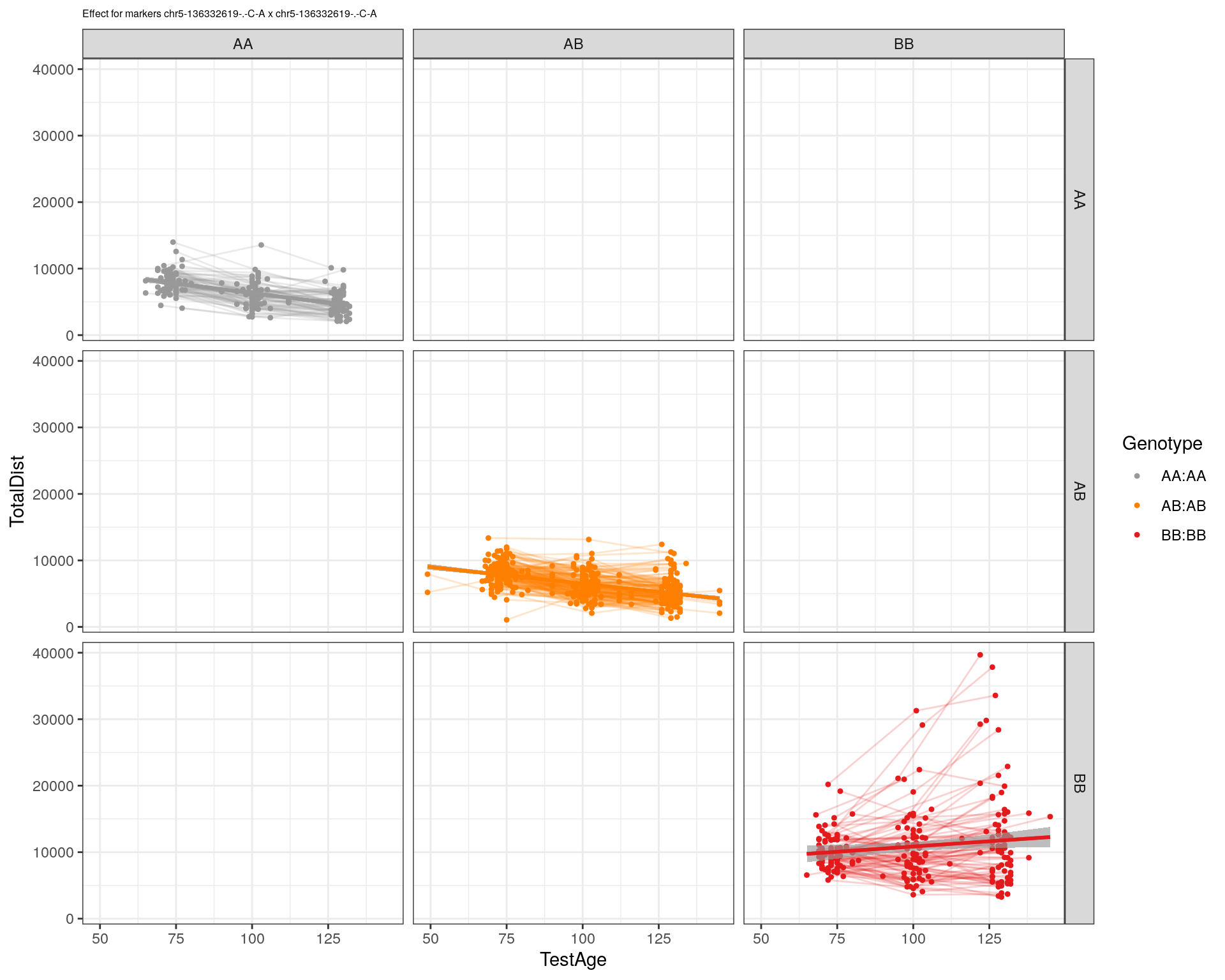
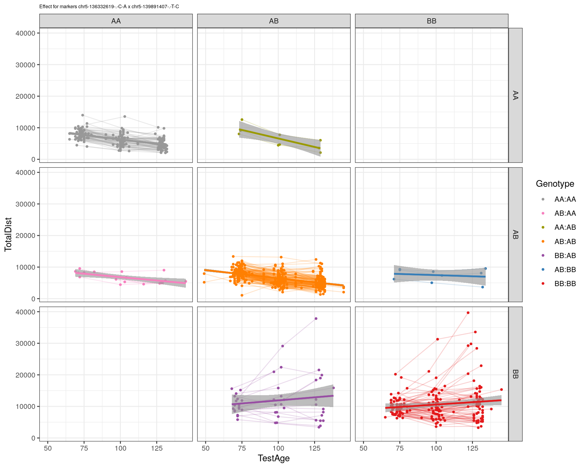
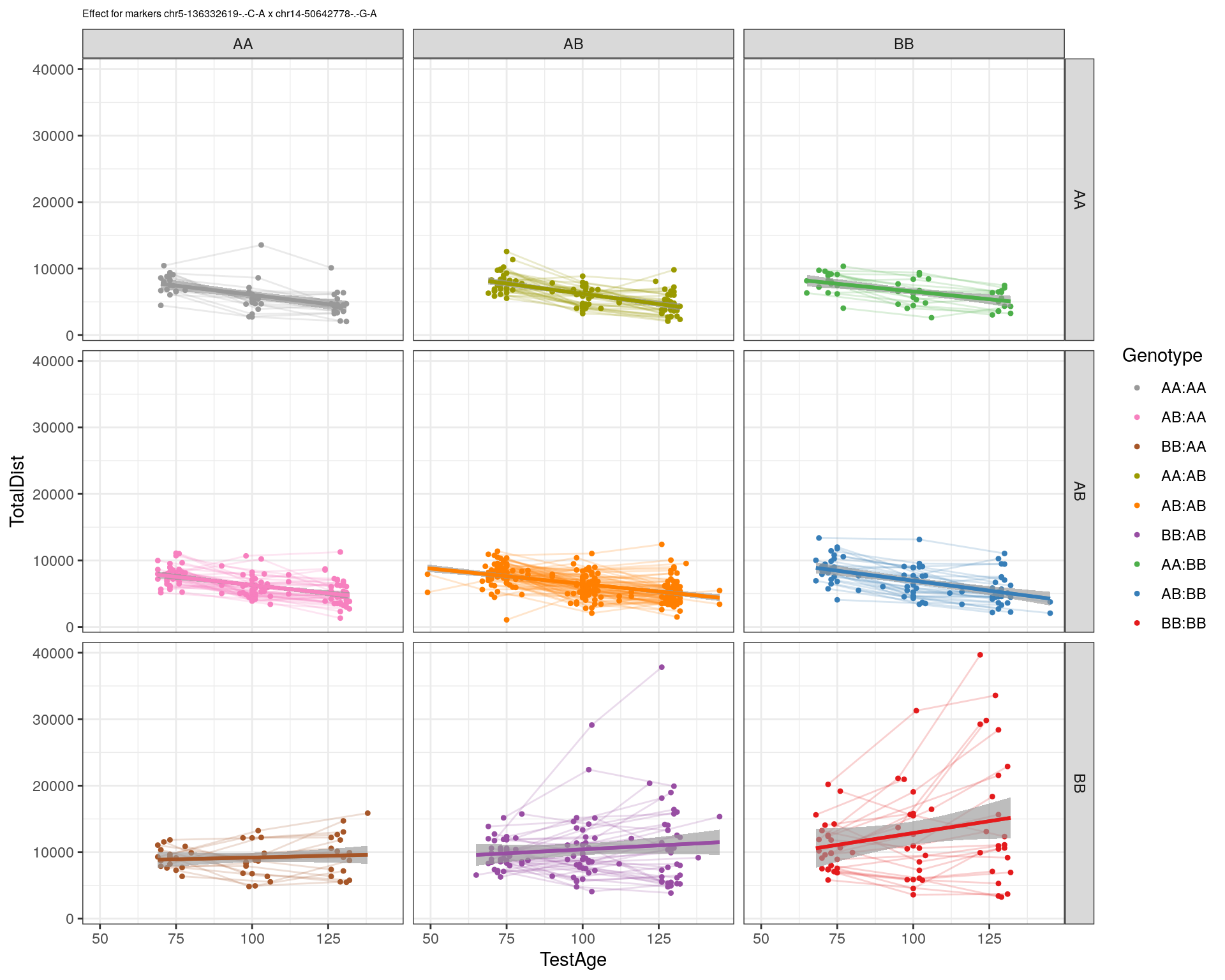
plot_int_graph <- function(cross, name,  basem){
  # Plot the Dist vs age, separate by genotype for each marker
  allphen <- cross$pheno
  allgeno <- as.data.frame(pull.geno(cross))
  rownames(allgeno) <- cross$pheno$AnimalName
  allphen <- merge(allphen, allgeno, by.x="AnimalName", by.y="row.names", all.x=TRUE)
  #pdf(paste0("output/", name, ".pdf"))
  for (mar in colnames(allgeno)){
    print(mar)
    subplot <- allphen[!is.na(allphen[,mar, drop=FALSE]),] %>% 
      pivot_longer(cols = starts_with("TestAge_"), names_to="test.no", values_to = "Age") %>% 
      separate(test.no, c("empty1", "test1")) %>%
      pivot_longer(cols = starts_with("TotalDist_"), names_to="test.no.2", values_to = "Dist") %>%
      separate(test.no.2, c("empty2", "test2")) %>% filter(test1==test2)
    subplot <- as.data.frame(subplot)
    subplot$interactions <- factor(subplot[, basem] + subplot[, mar]*3)
    # 1:1 -> 4 1:2 -> 7 1:3 -> 10
    # 2:1 -> 5 2:2 -> 8 2:3 -> 11
    # 3:1 -> 6 3:2 -> 9 3:3 -> 12
    itypes  <- c(1,2,3,"AA:AA", "AB:AA", "BB:AA", 
                "AA:AB", "AB:AB", "BB:AB",
                "AA:BB", "AB:BB", "BB:BB")
    levels(subplot$interactions) <- itypes[as.integer(levels(subplot$interactions))]
    
    #replaces 1 2 and 3 as AA, AB and BB
    subplot[, basem][subplot[, basem] == 1] <- "AA"
    subplot[, basem][subplot[, basem] == 2] <- "AB"
    subplot[, basem][subplot[, basem] == 3] <- "BB"
    subplot[, mar][subplot[, mar] == 1] <- "AA"
    subplot[, mar][subplot[, mar] == 2] <- "AB"
    subplot[, mar][subplot[, mar] == 3] <- "BB"
    
    p1 <- ggplot(subplot, aes(Age, Dist, color=interactions, group=interactions)) + 
      geom_point(shape = 20) + 
      #scale_color_discrete("Genotype") +
      labs(color = "Genotype") +
      ylab("TotalDist") +
      xlab("TestAge") +
      #scale_color_brewer(palette = "Set1") + 
      scale_color_manual(breaks = c("AA:AA", "AB:AA", "BB:AA", "AA:AB",
                                    "AB:AB", "BB:AB", "AA:BB", "AB:BB", "BB:BB"),
                                         #values = RColorBrewer::brewer.pal(9, "Set1")[9:1]) +
                       values = c("#999999", "#F781BF", "#A65628","#9a9a00", "#FF7F00", "#984EA3", "#4DAF4A", "#377EB8", "#E41A1C")) +
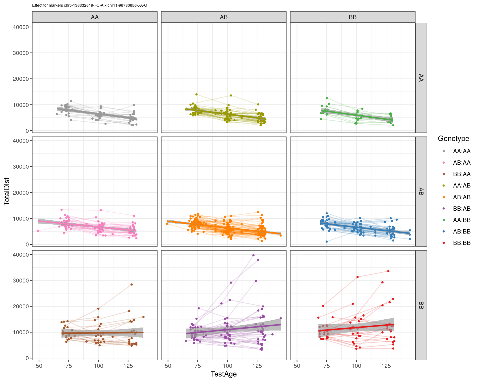
      stat_smooth(method="lm", show.legend = FALSE, formula = y~x) + 
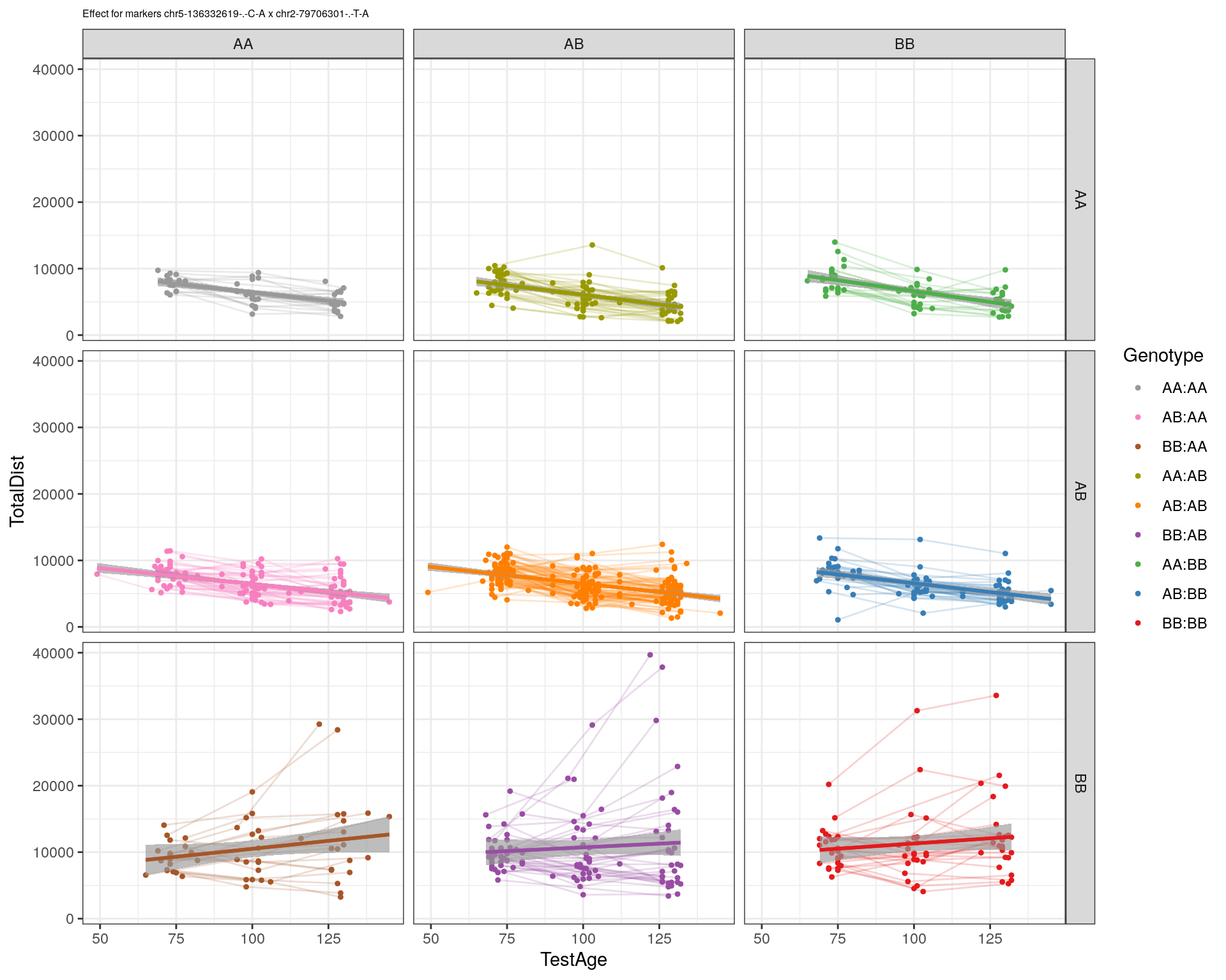
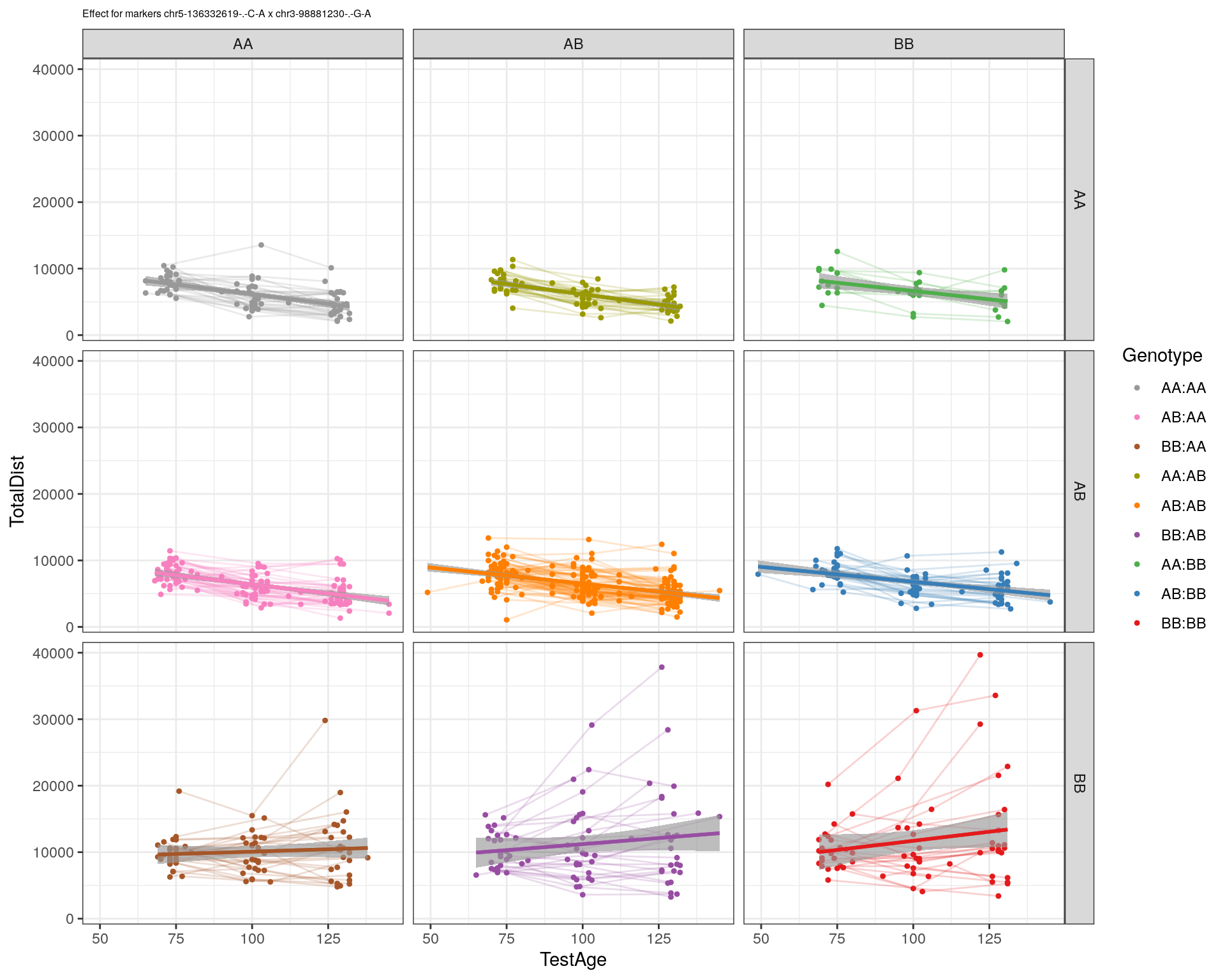
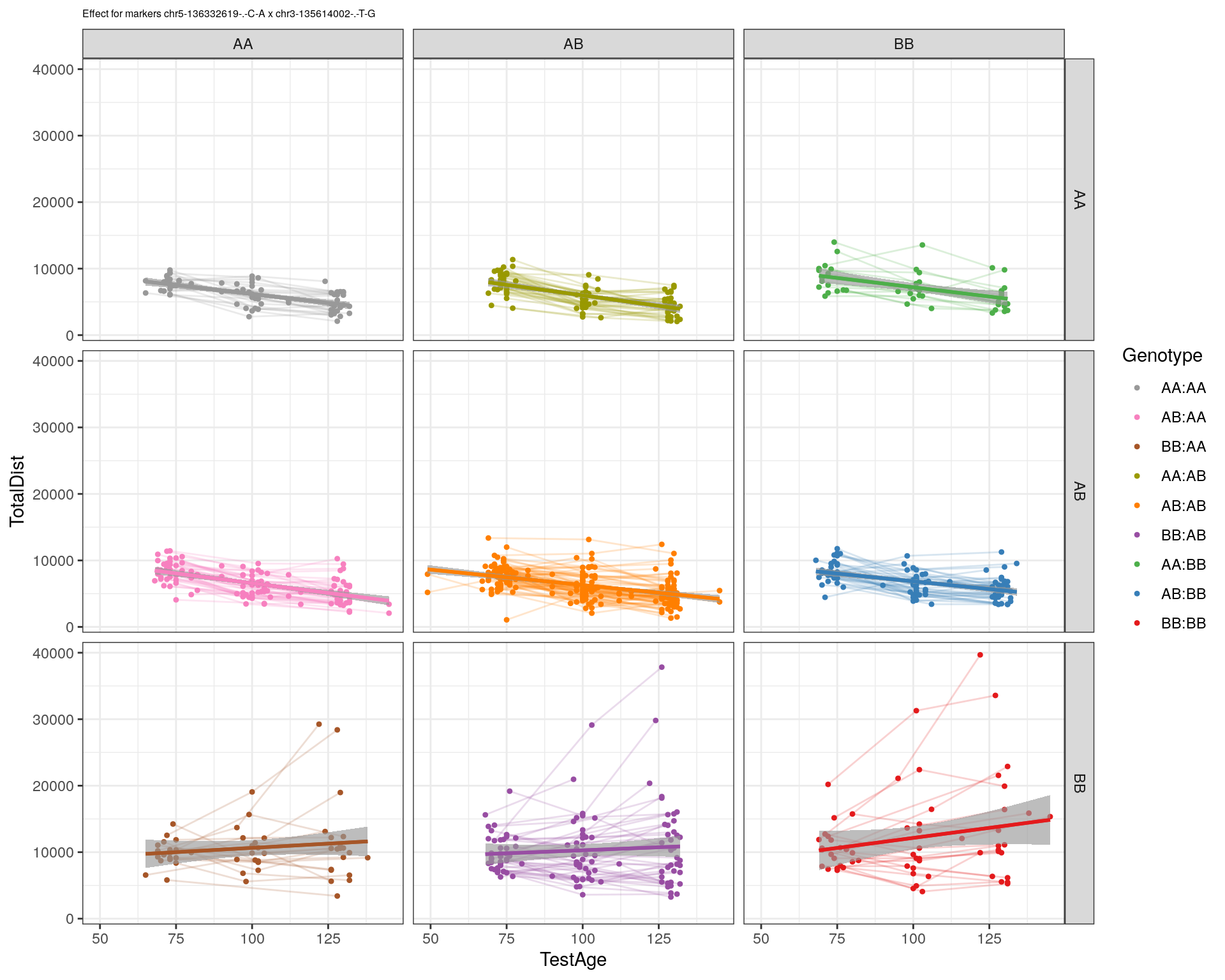
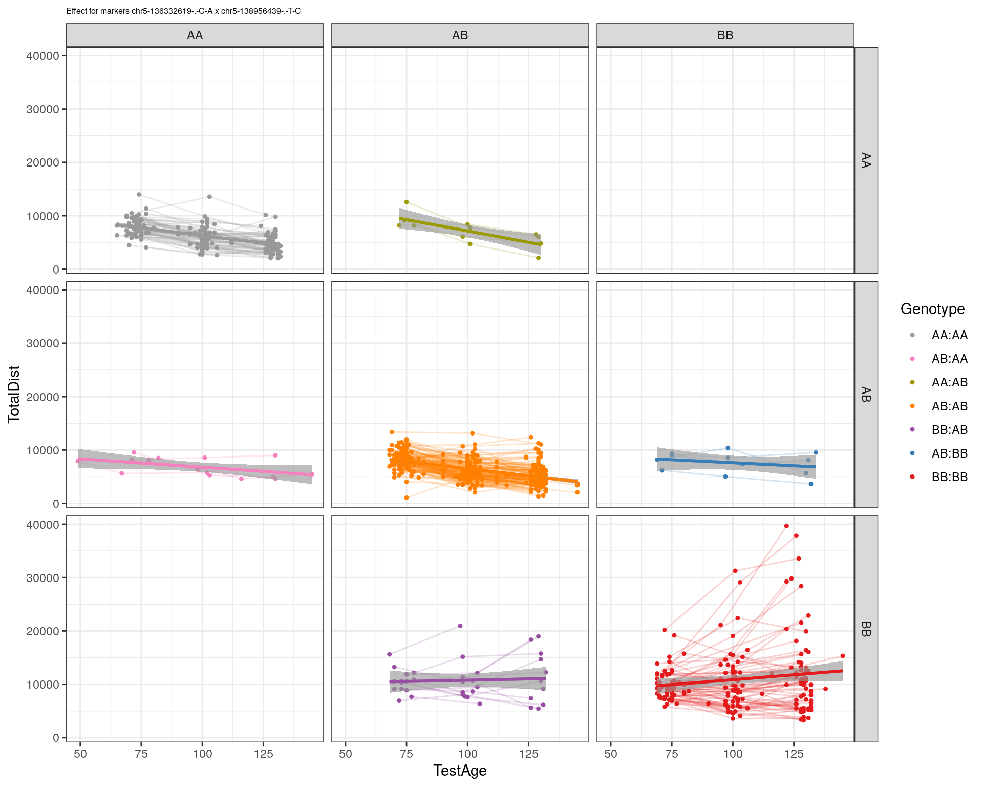
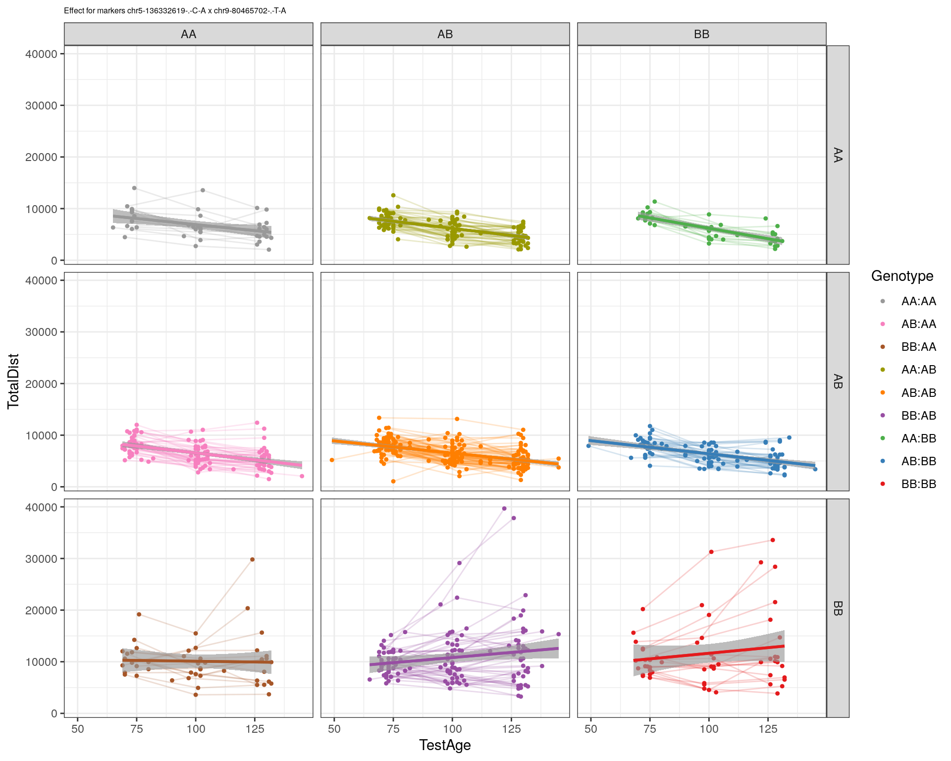
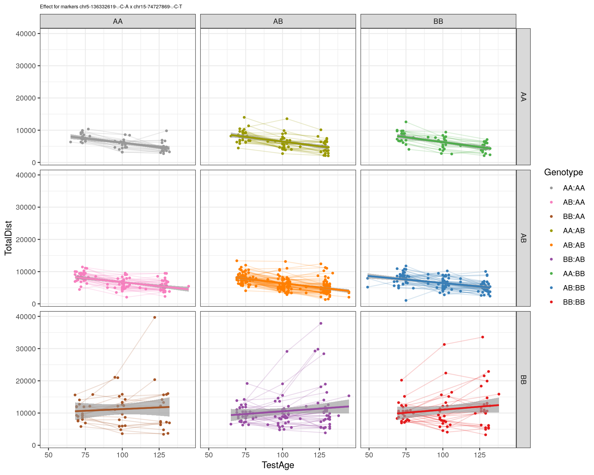
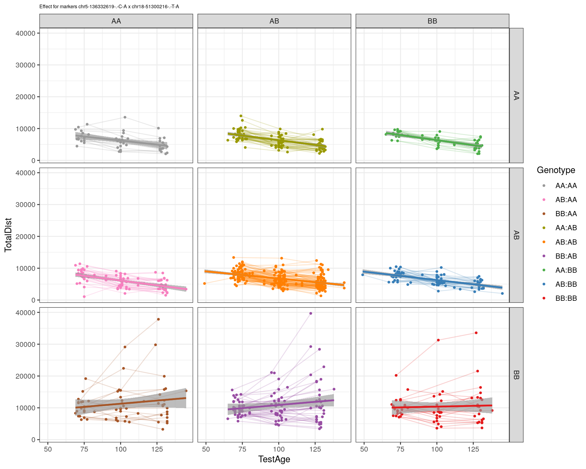
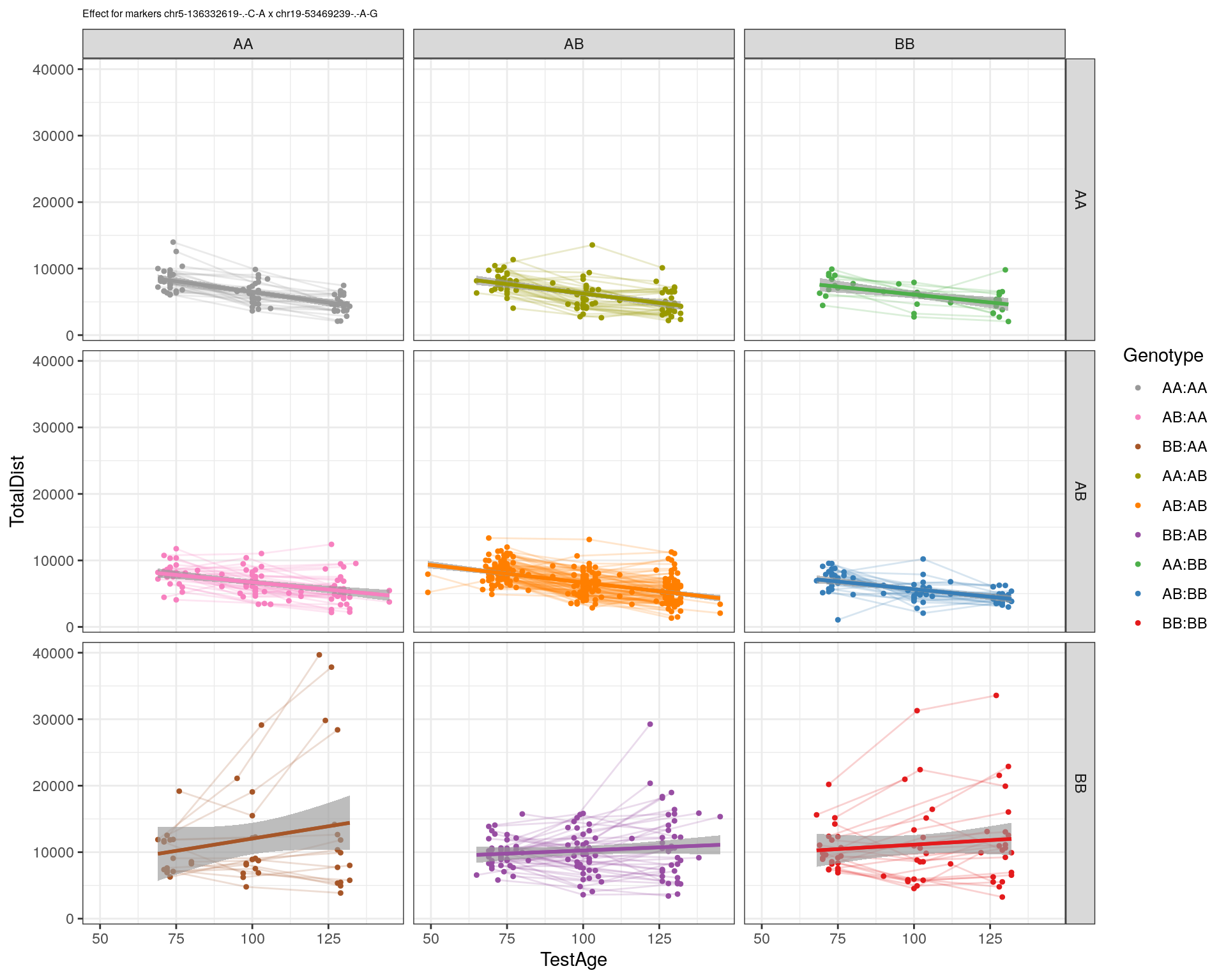
      labs(title=paste0("effect for markers ", basem, " x ", mar)) +
      theme_bw()
    print(p1)
    
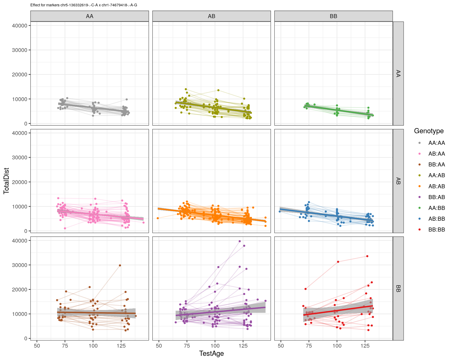
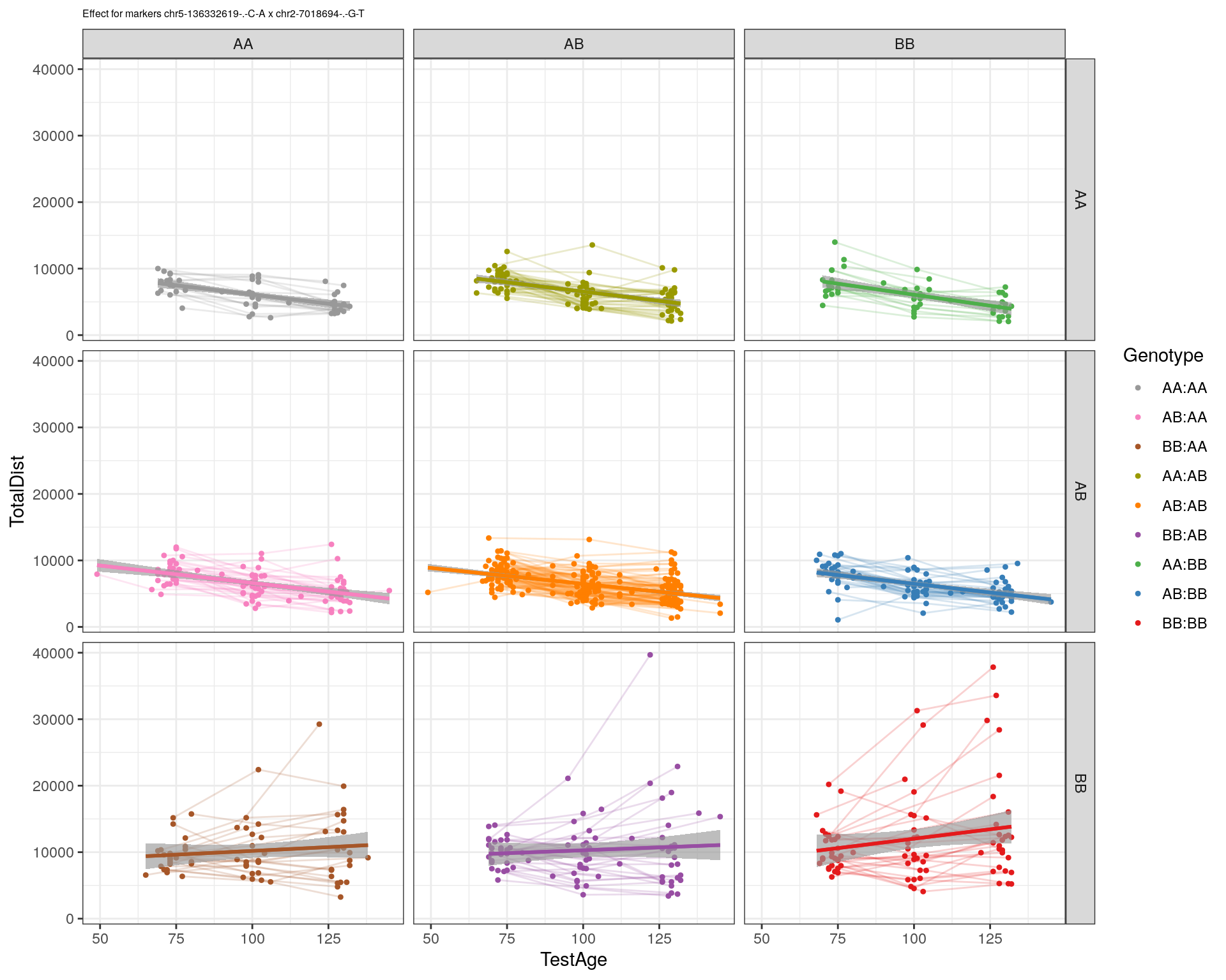
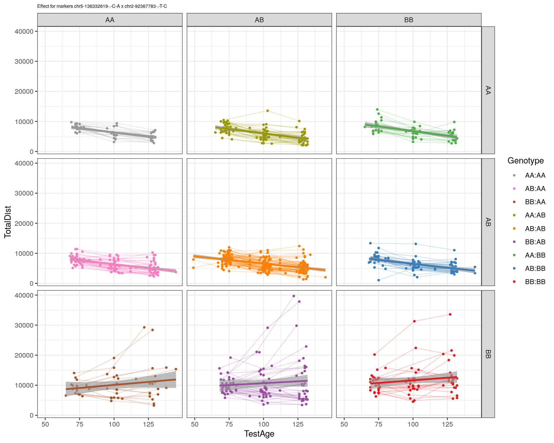
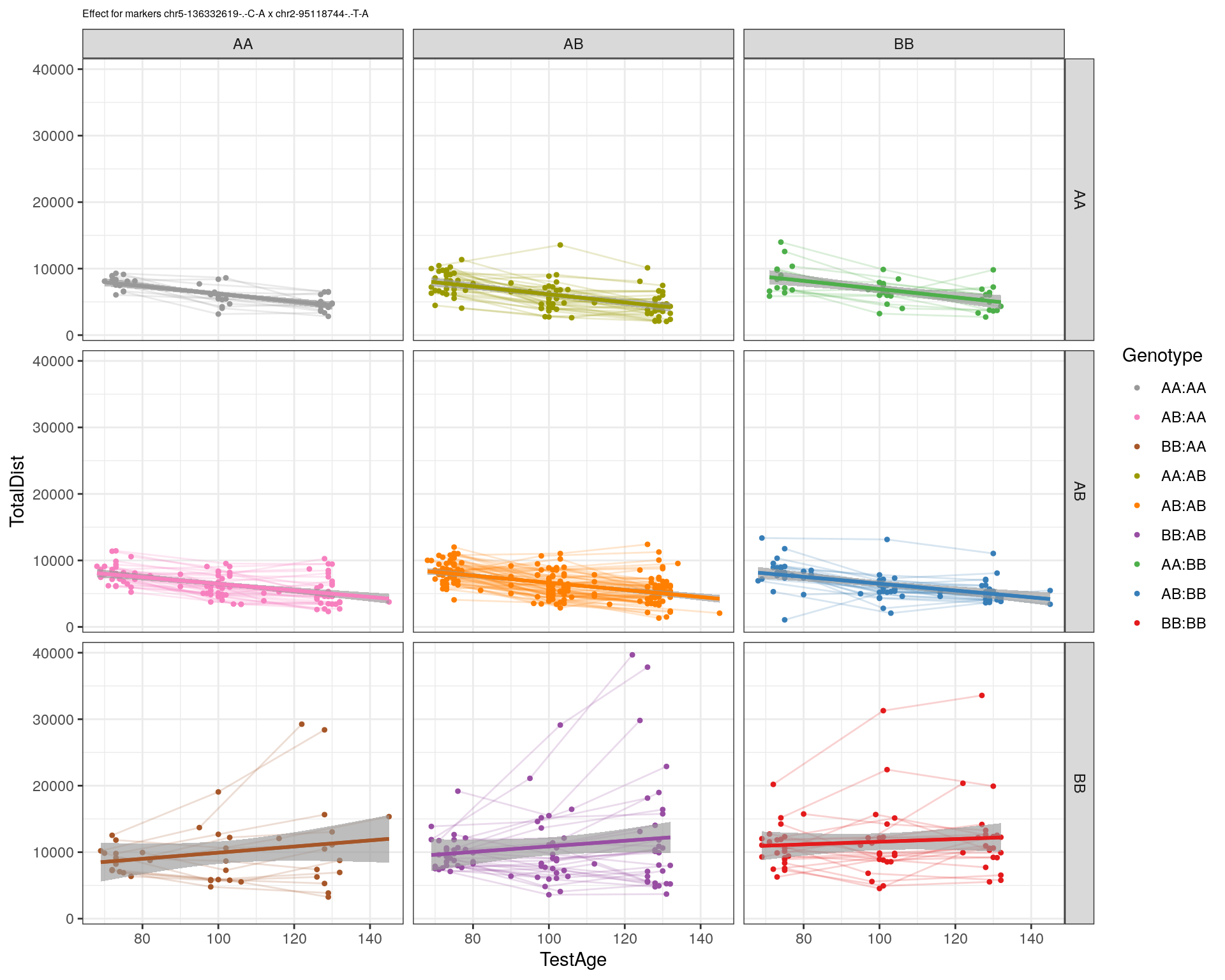
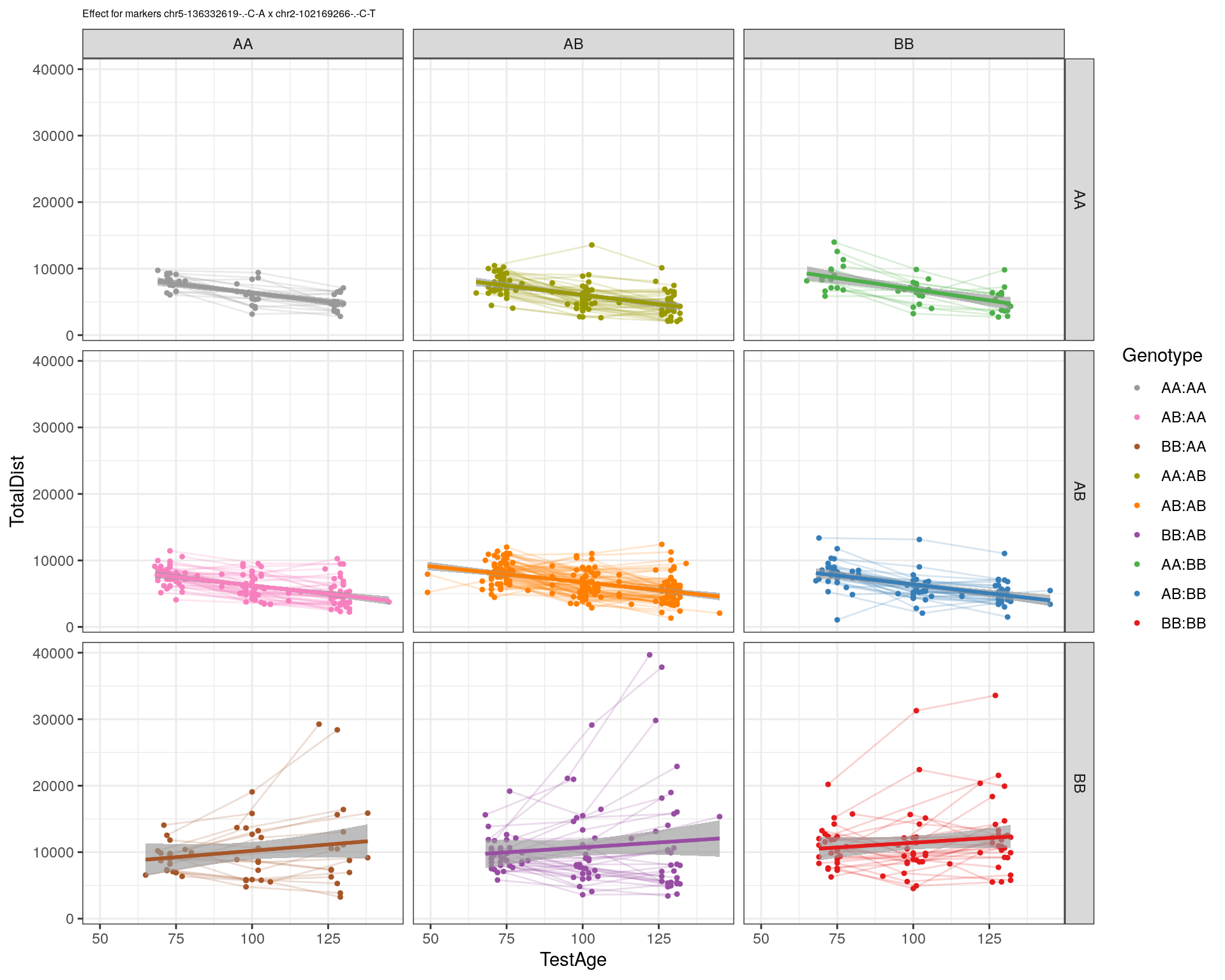
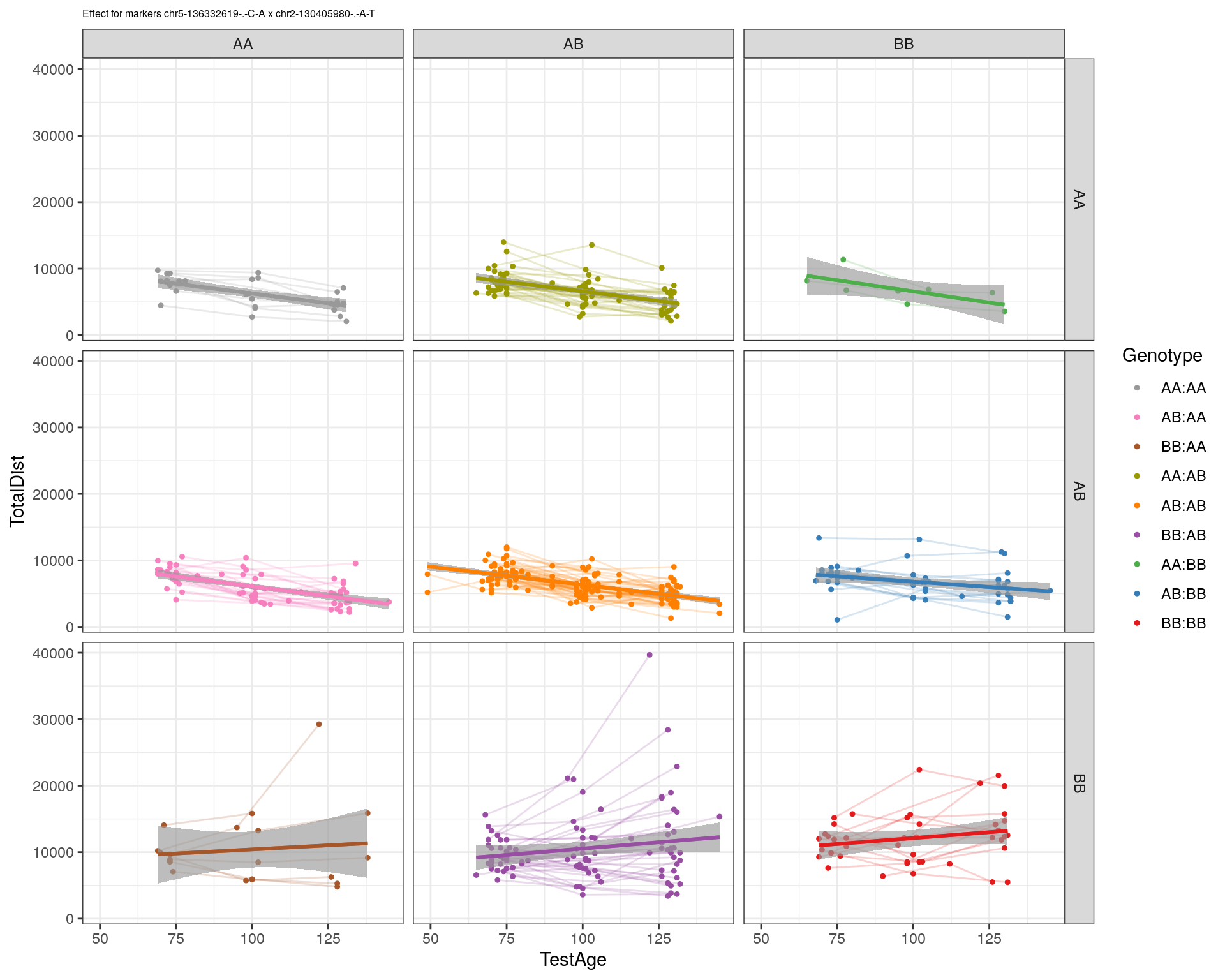
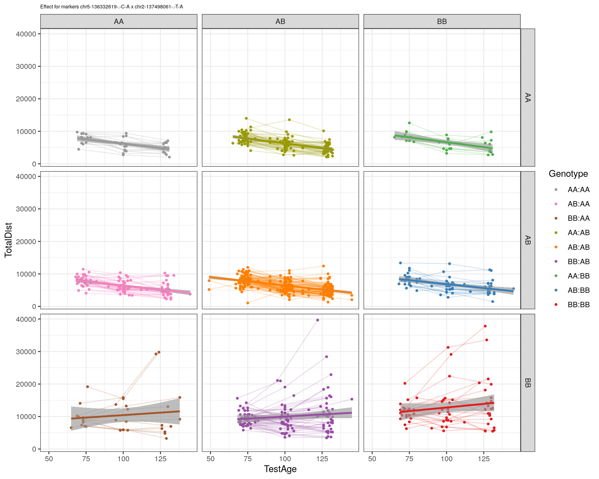
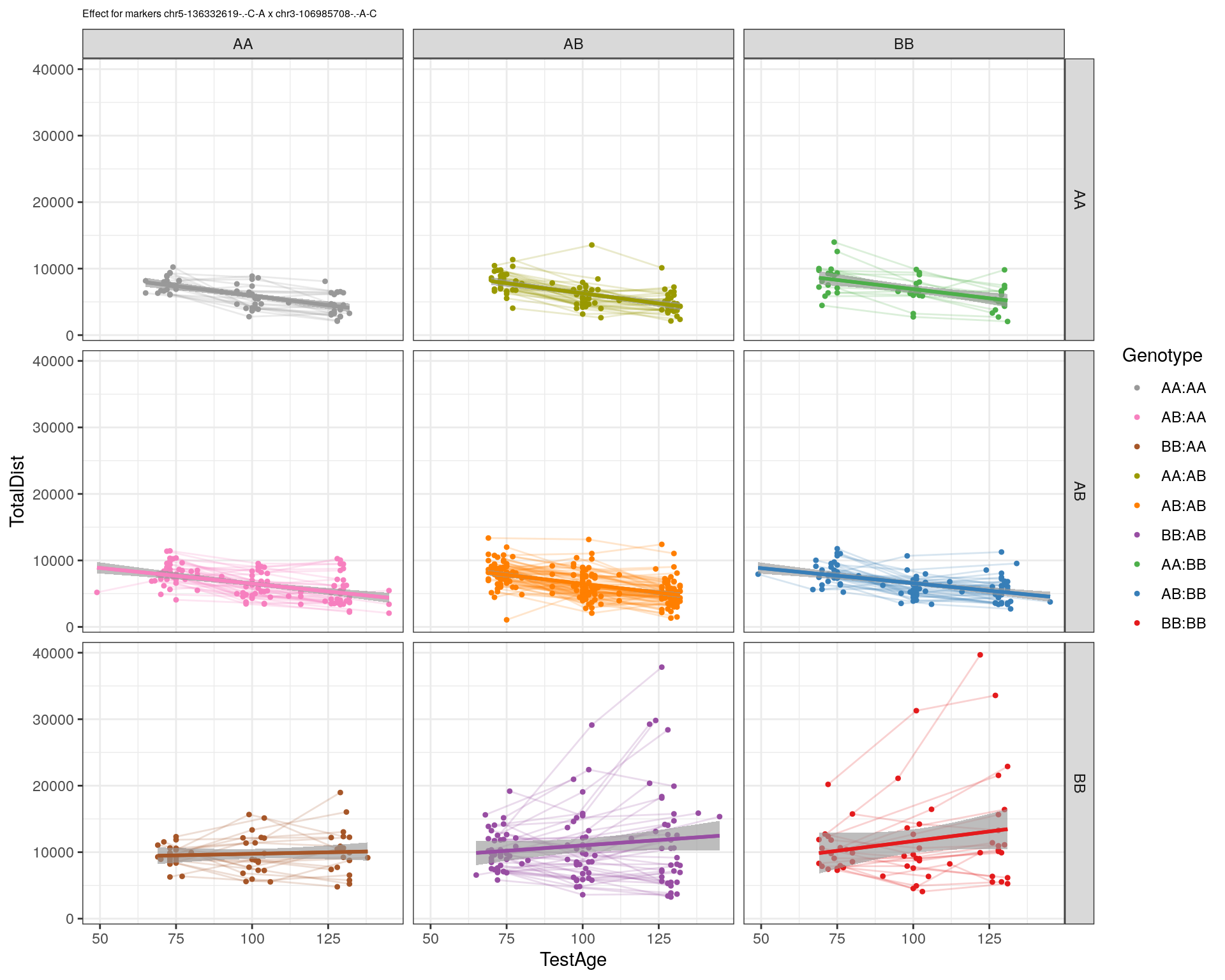
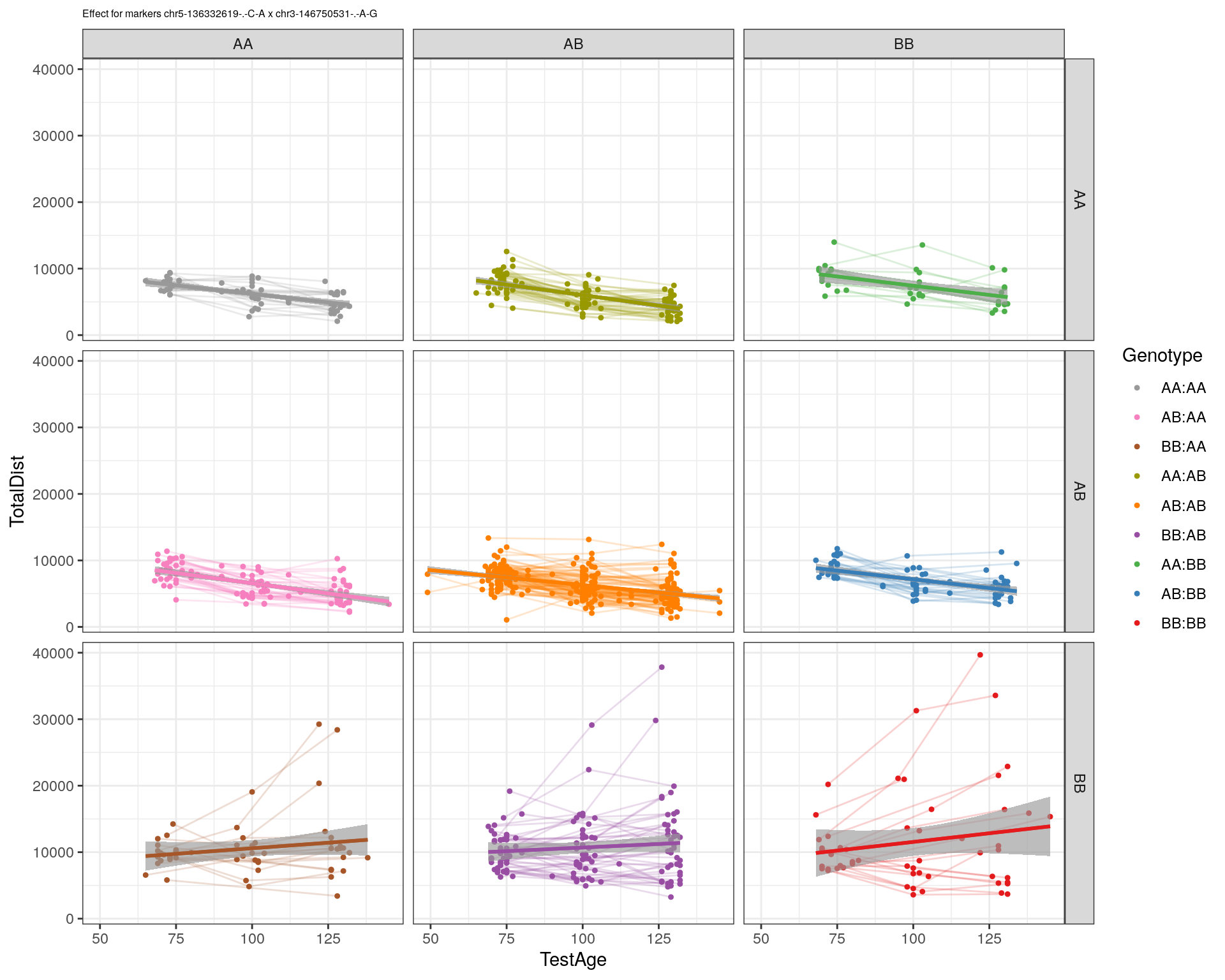
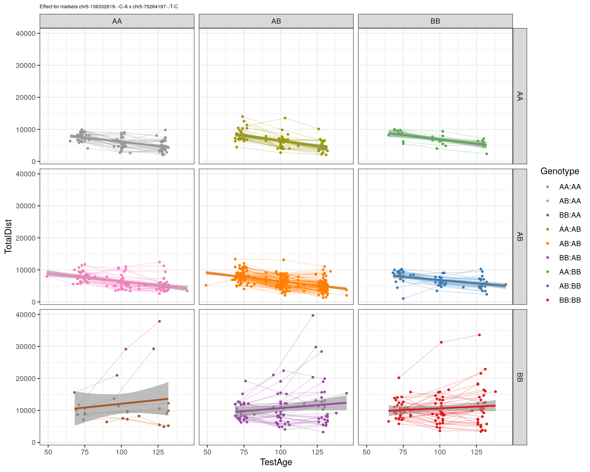
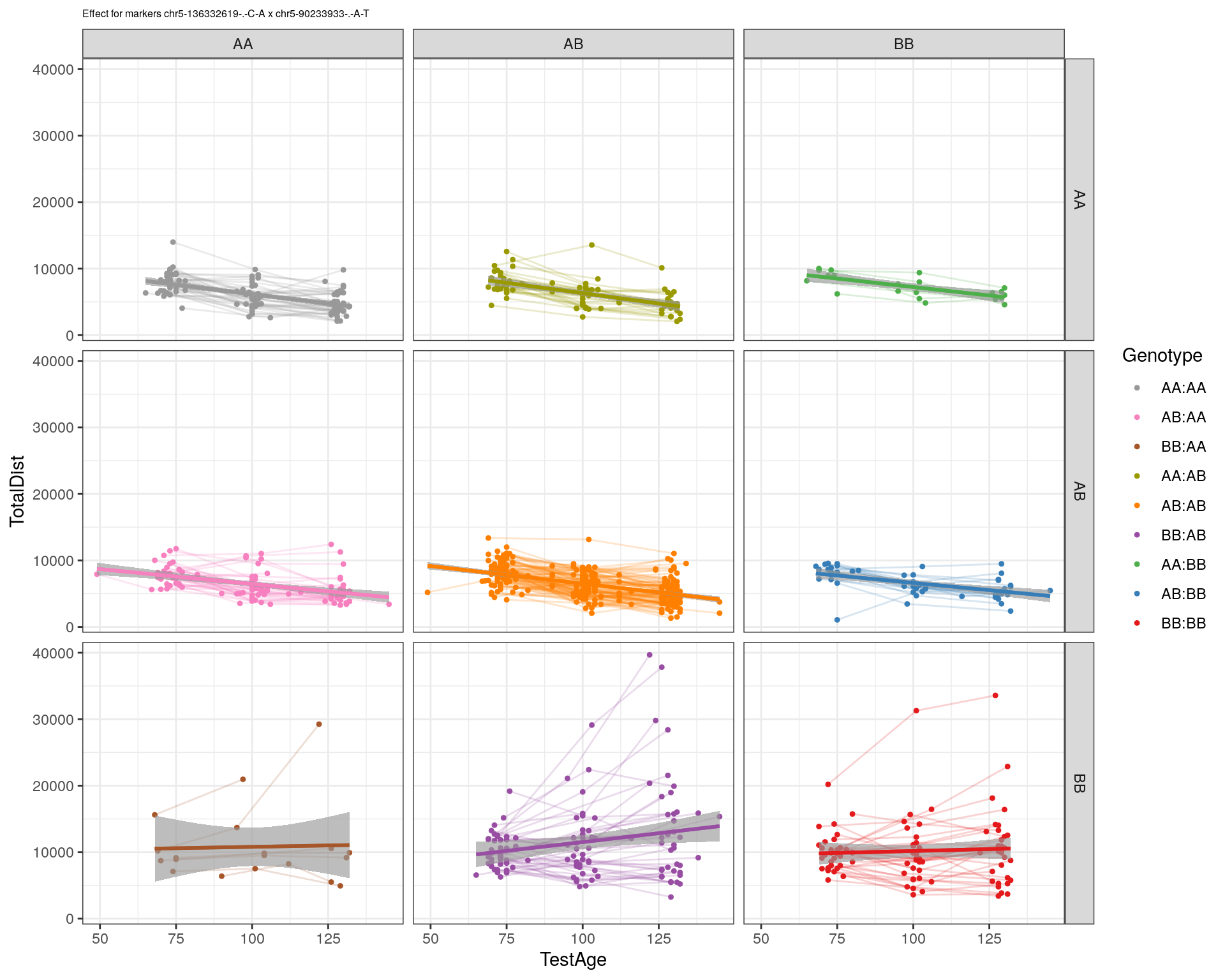
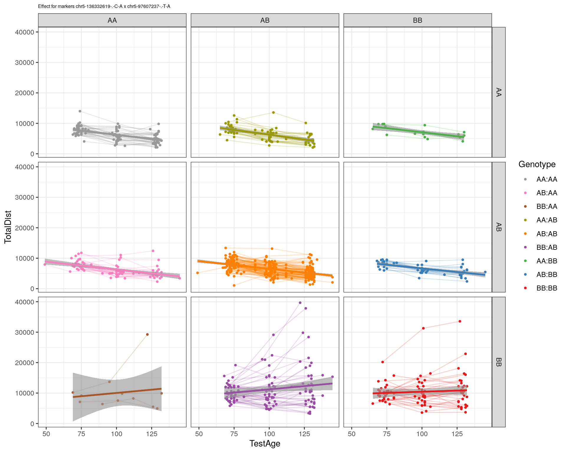
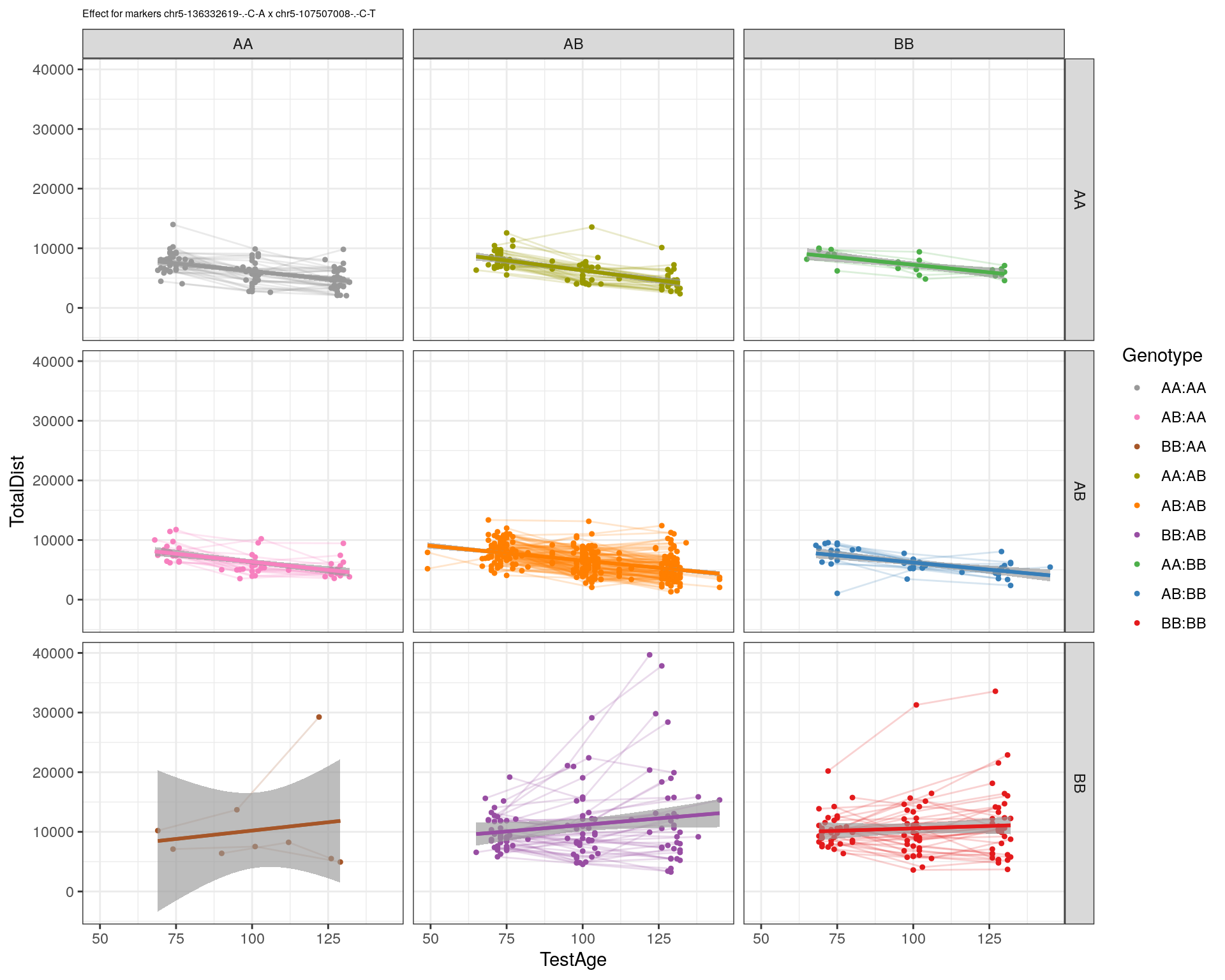
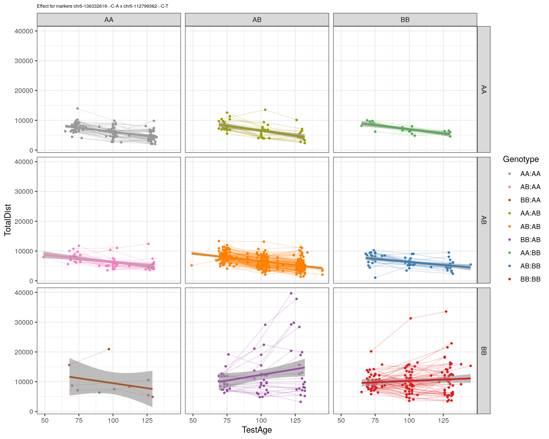
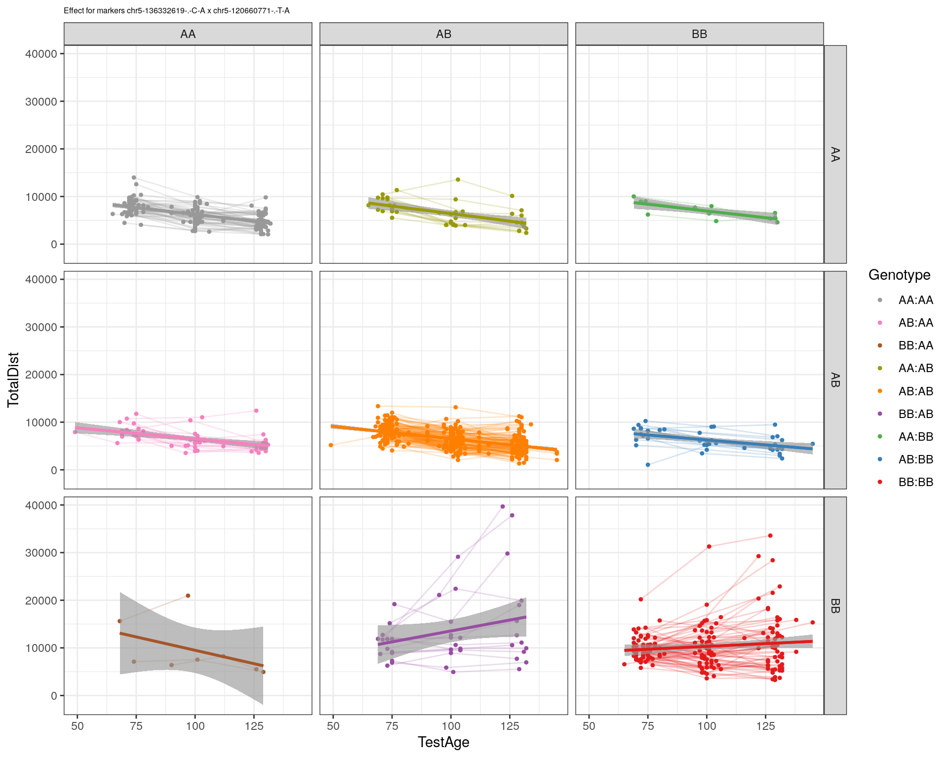
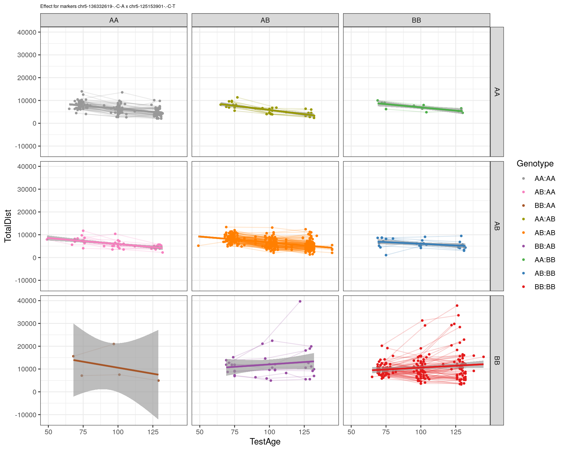
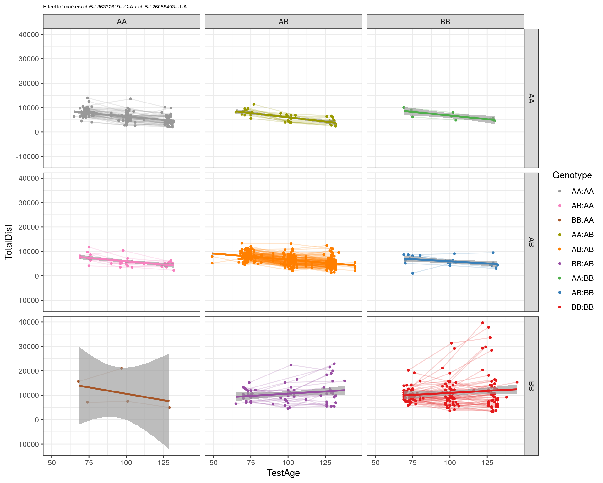
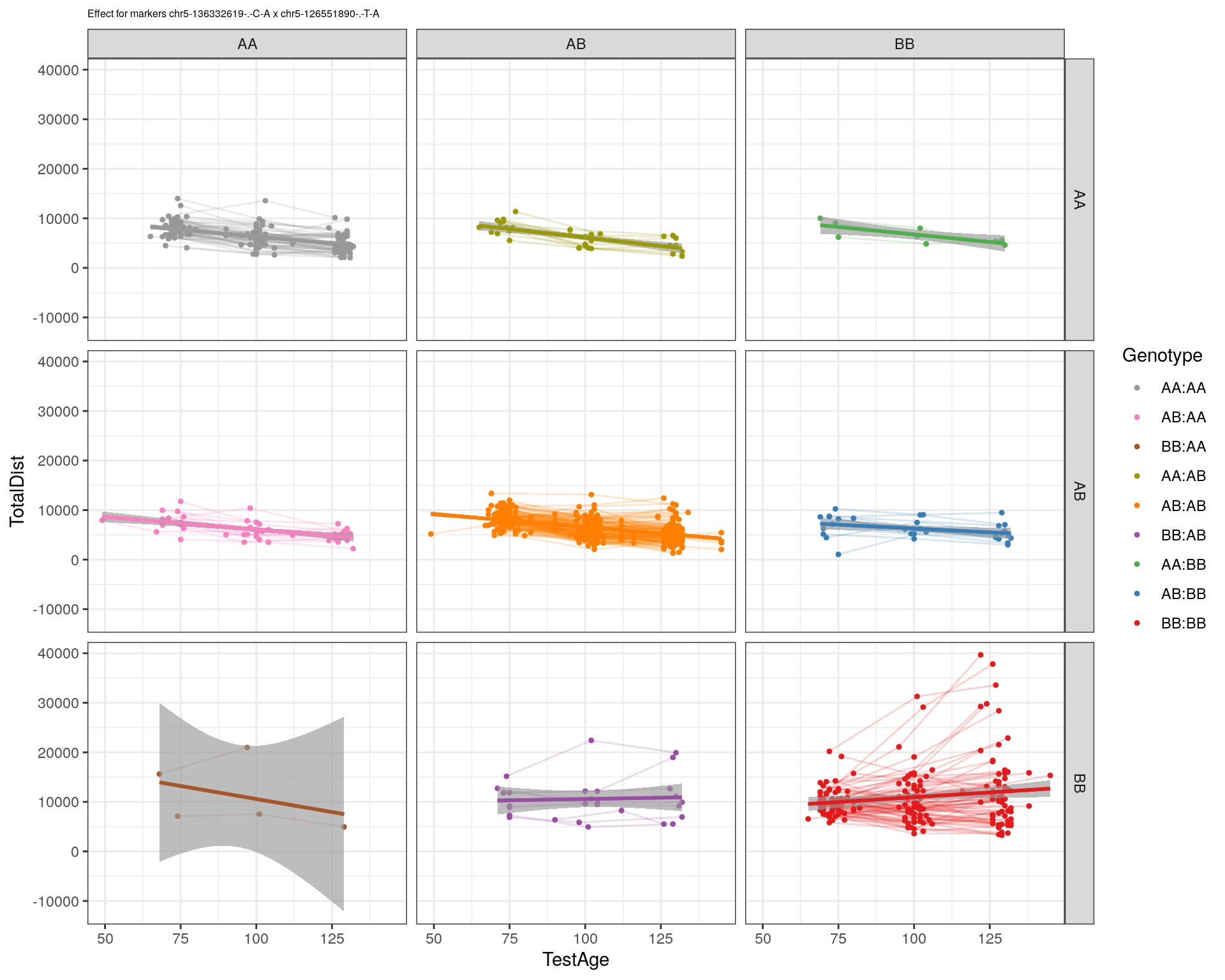
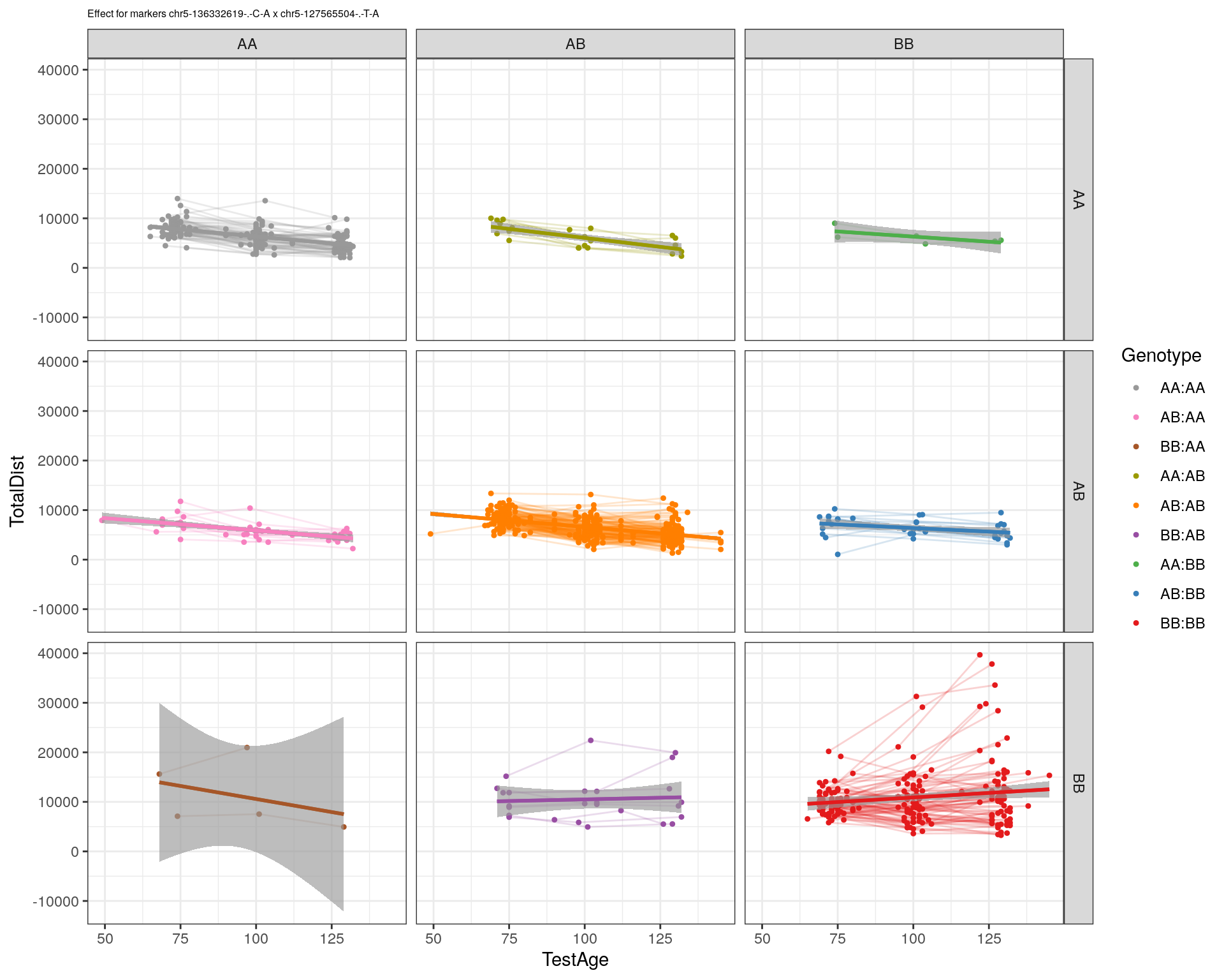
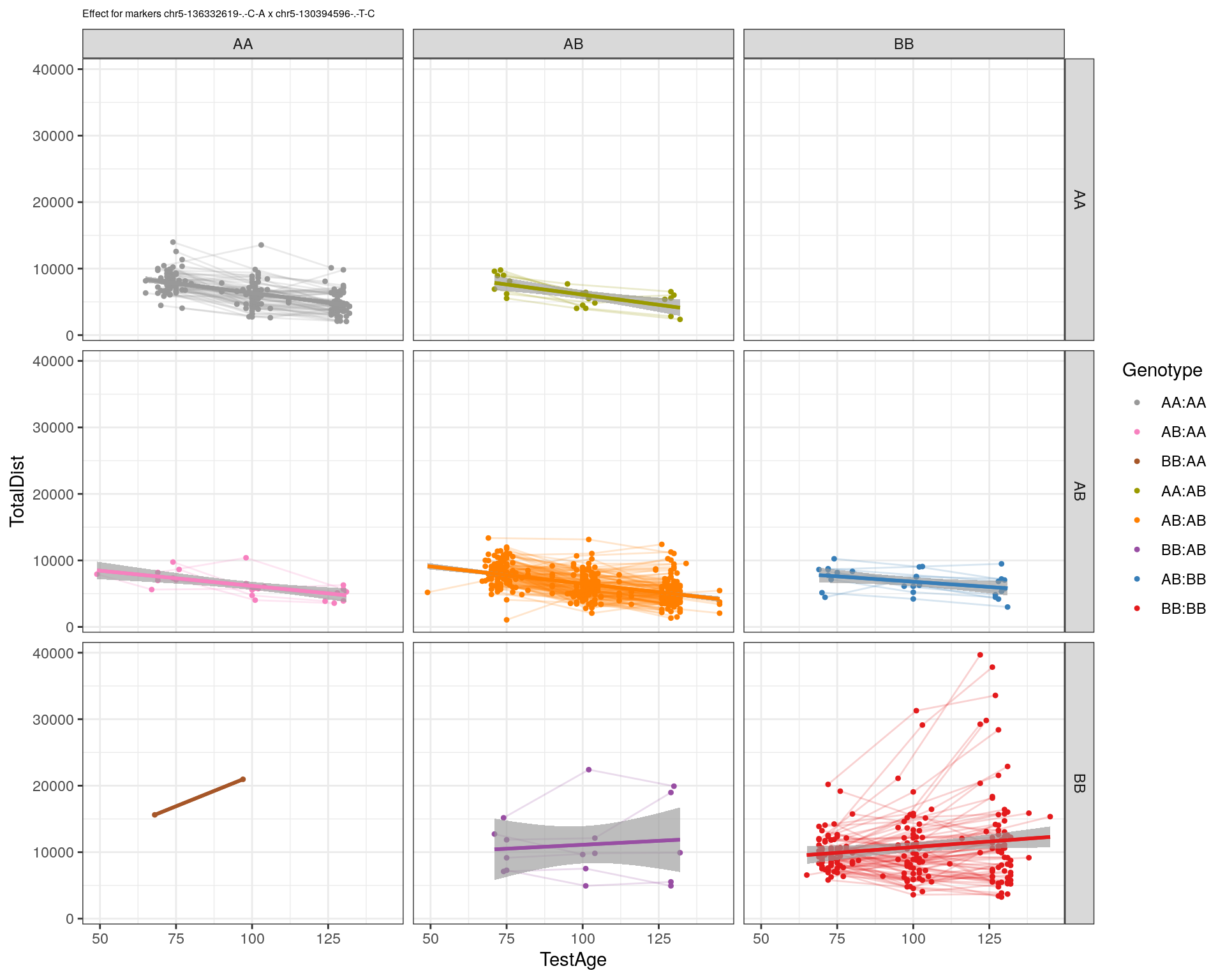
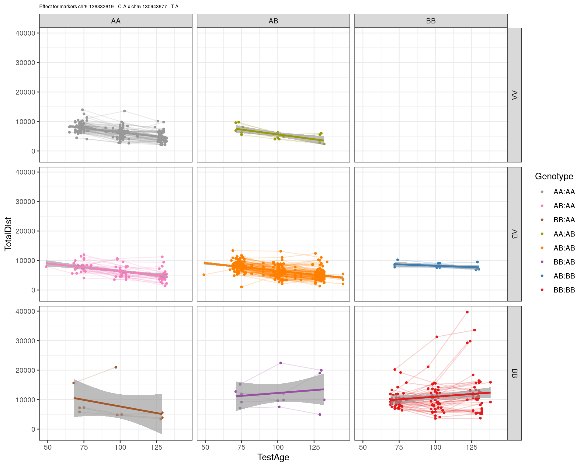
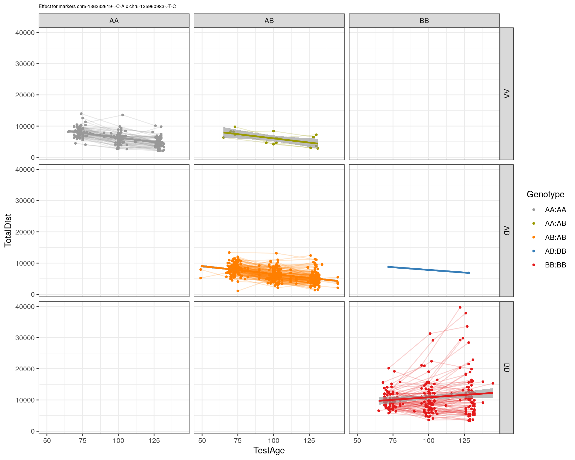
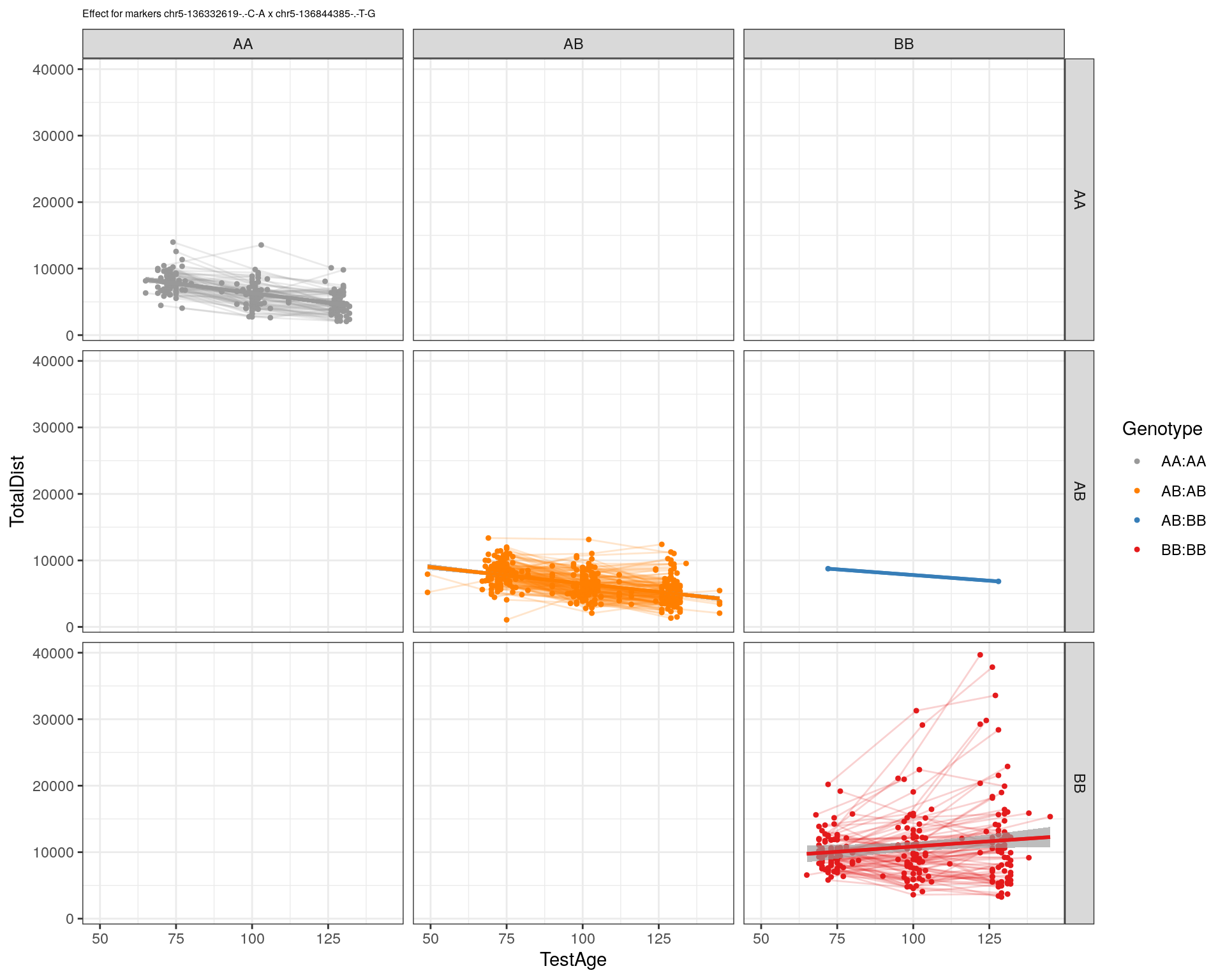
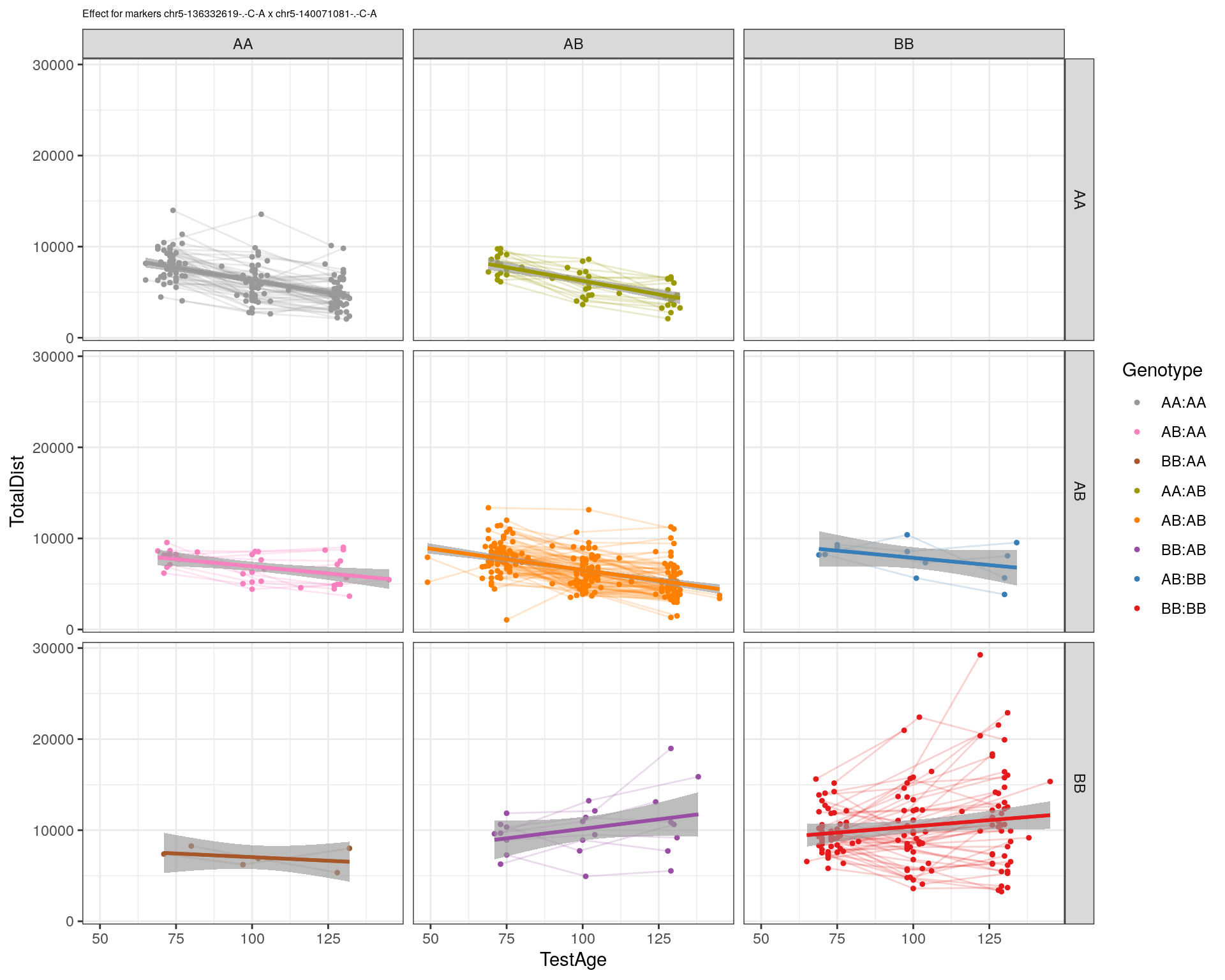
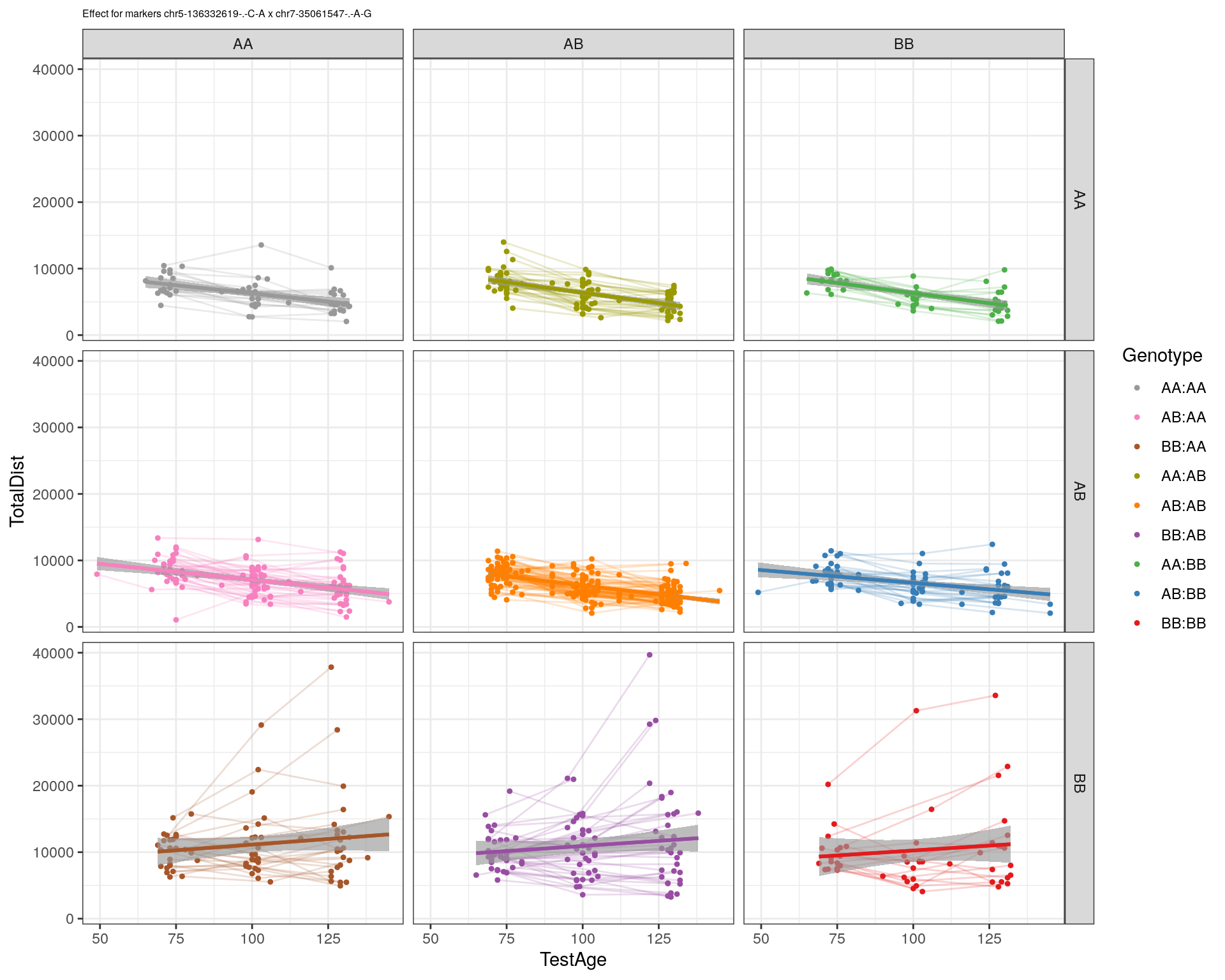
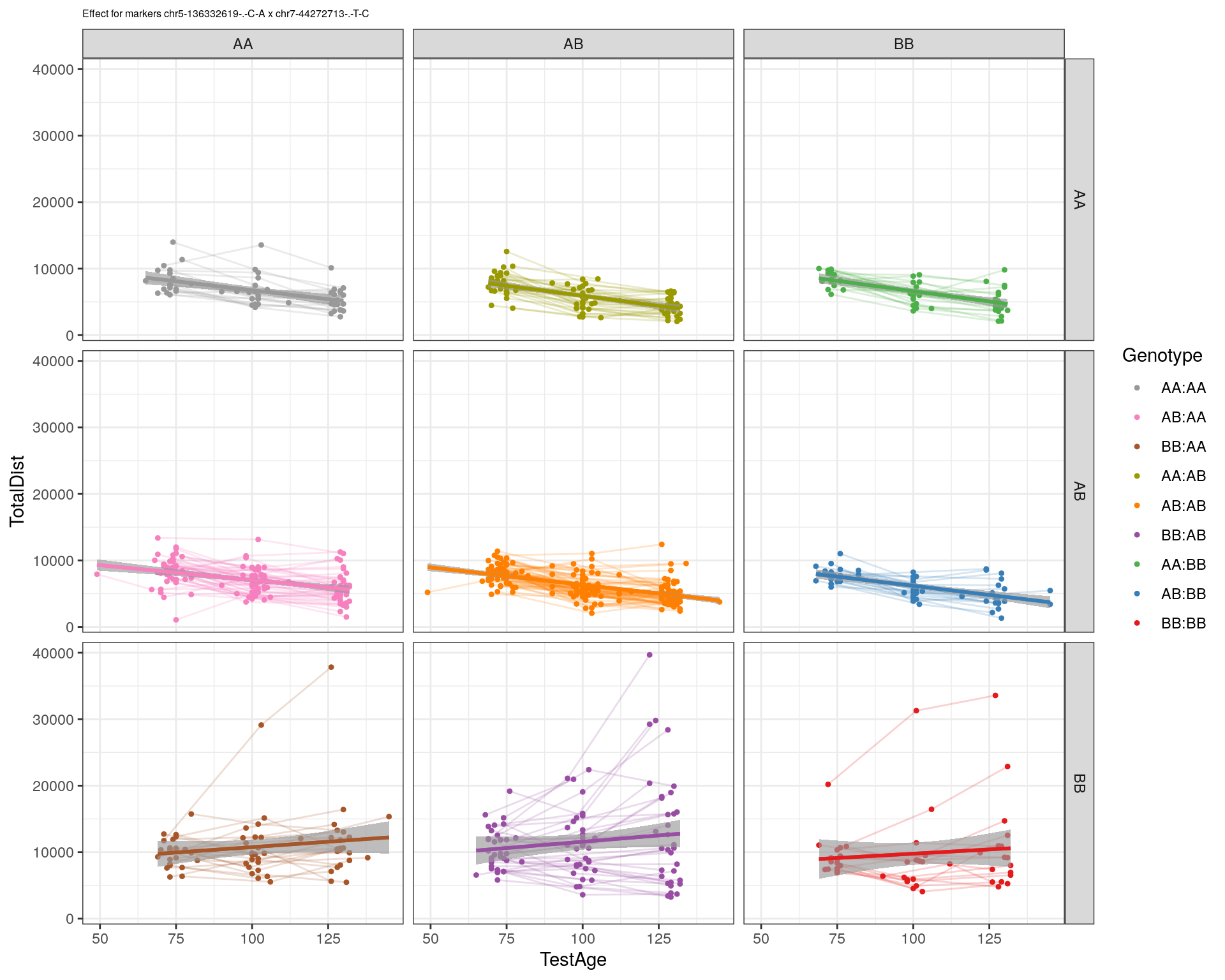
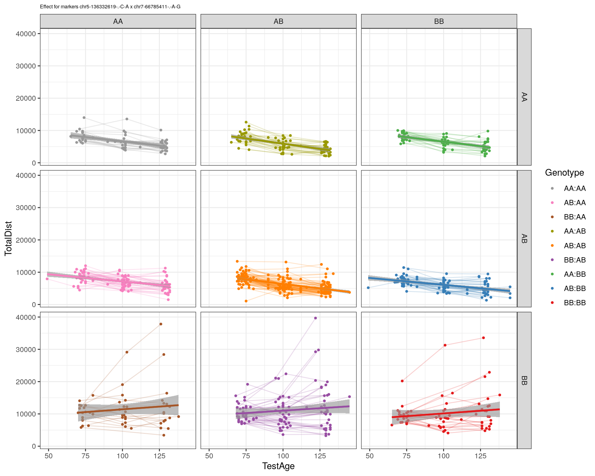
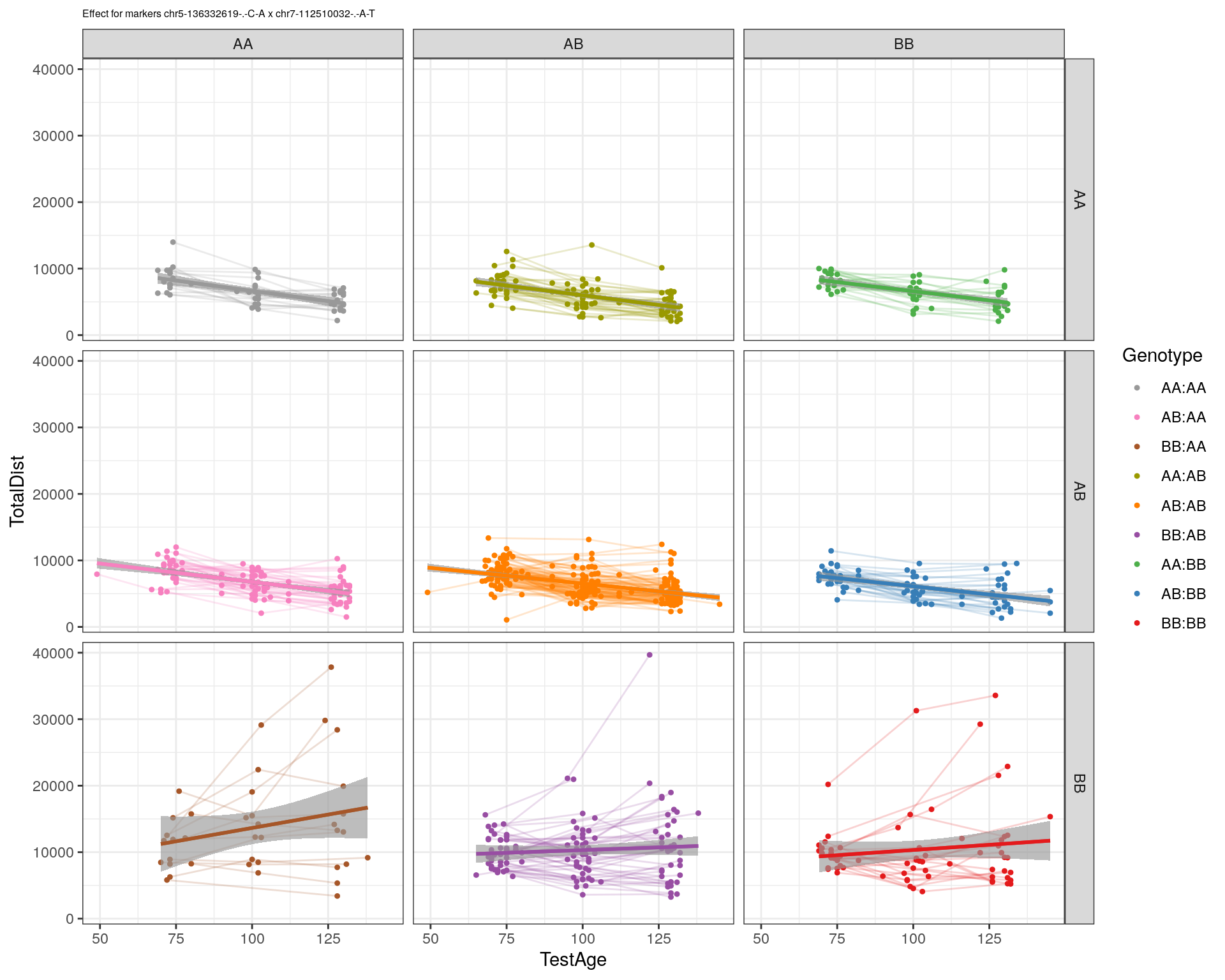
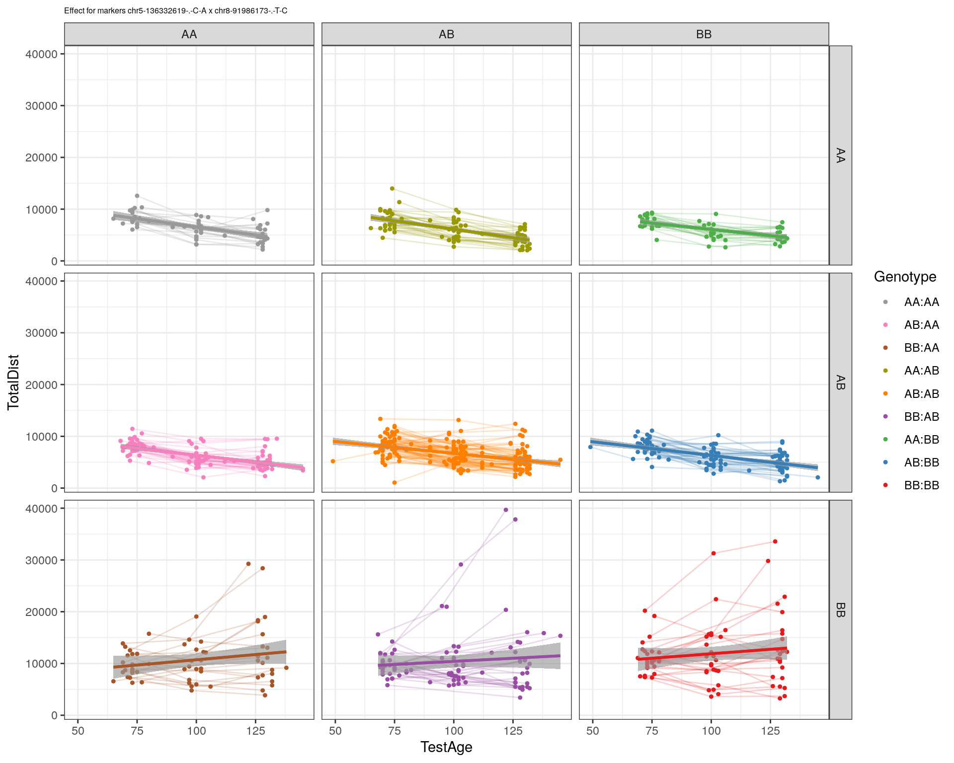
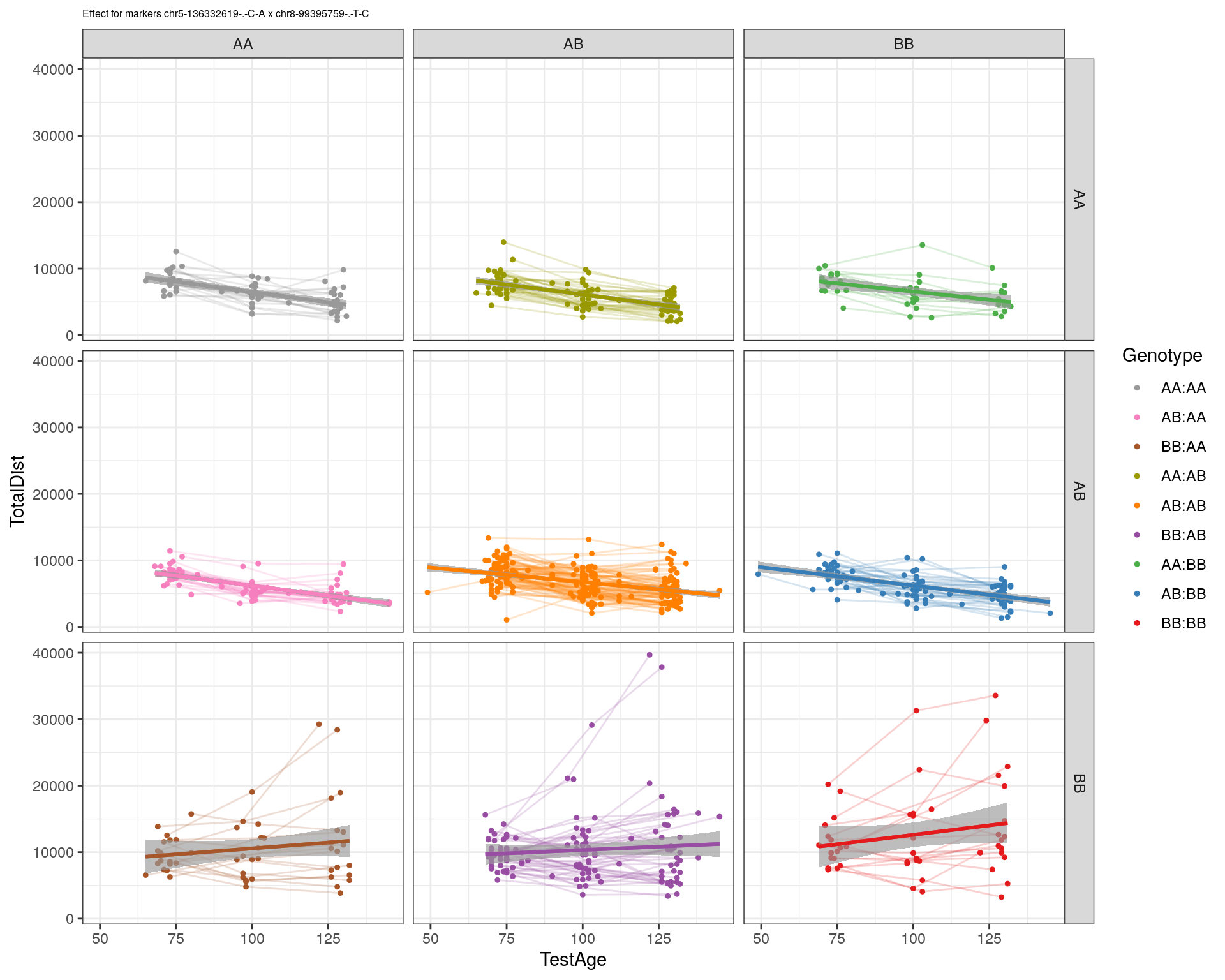
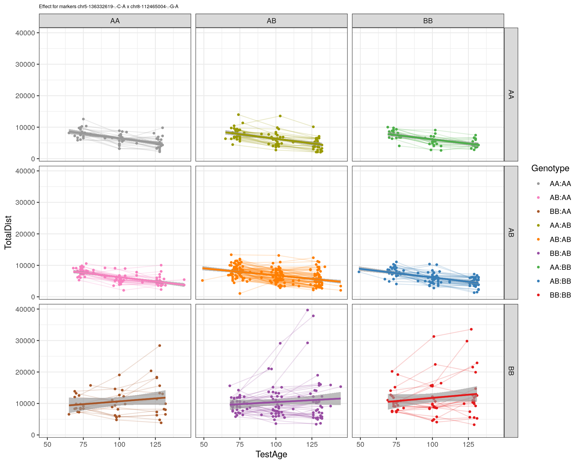
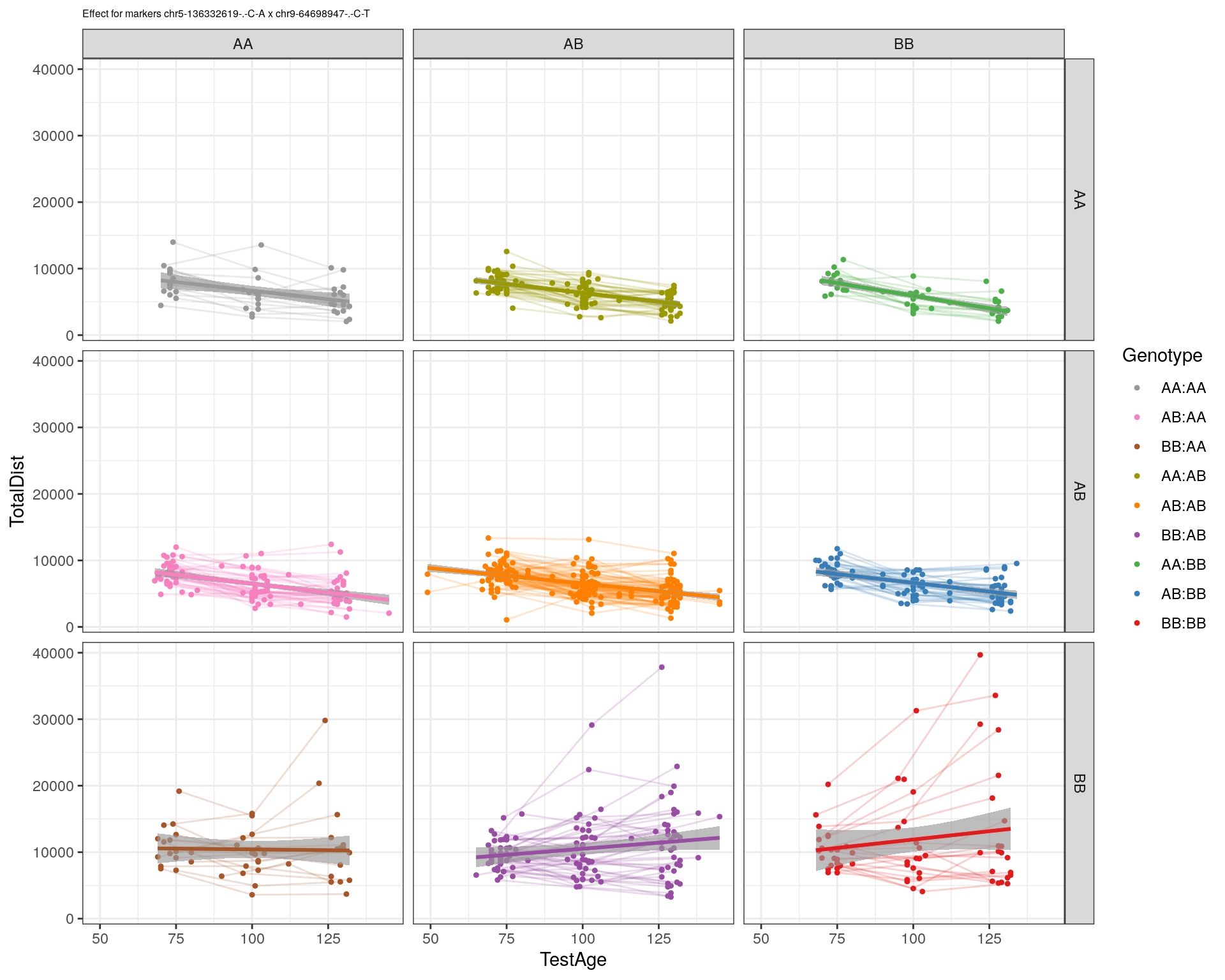
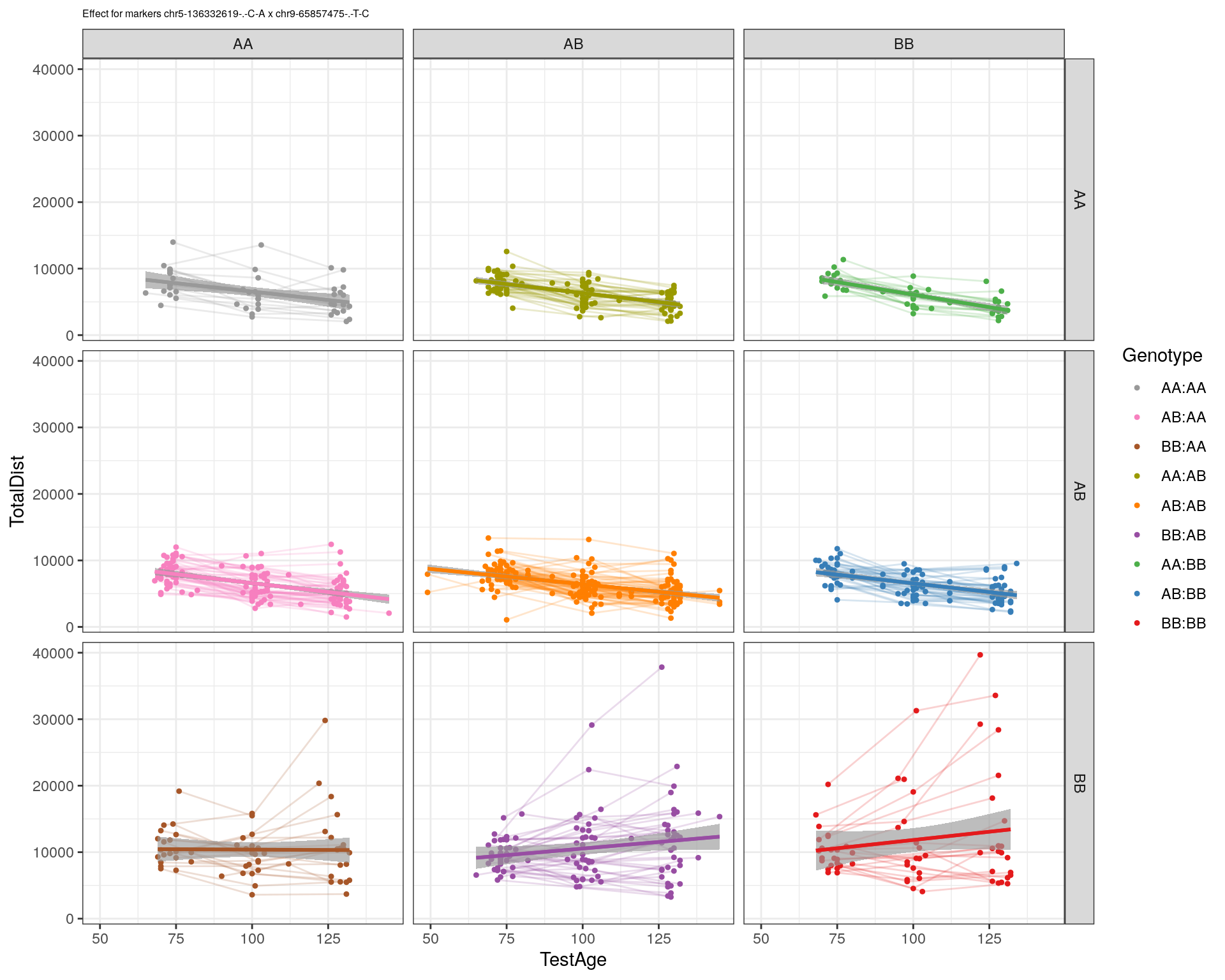
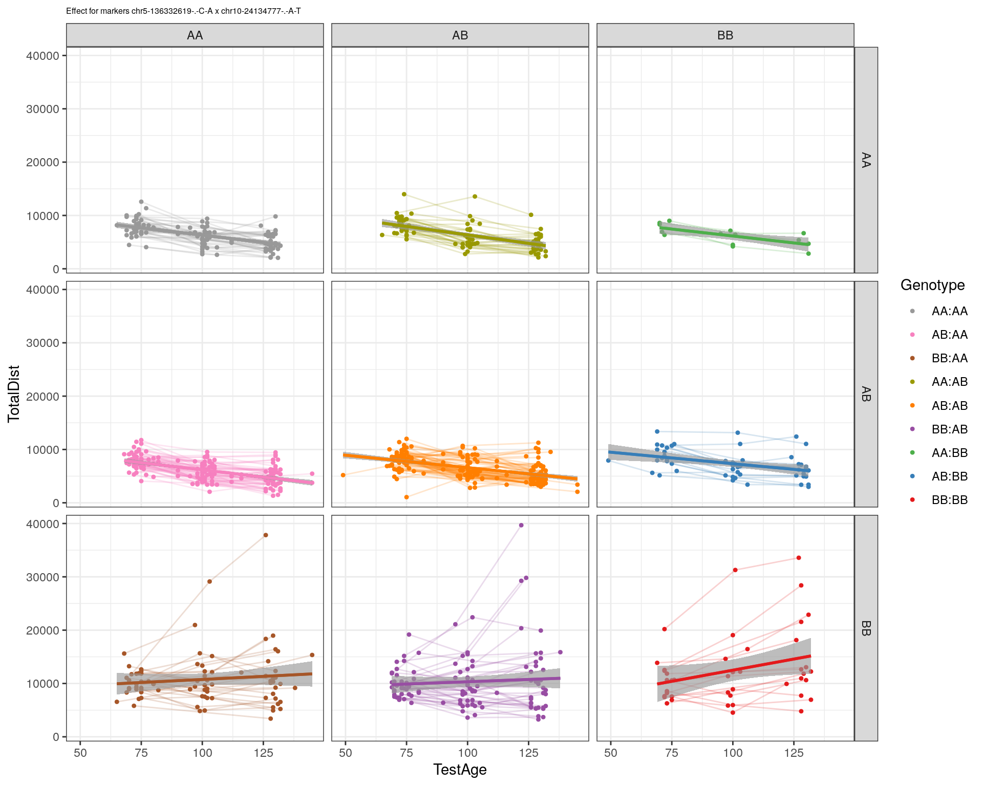
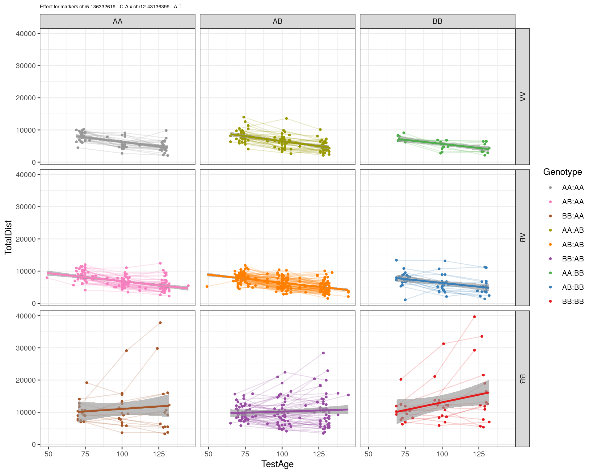
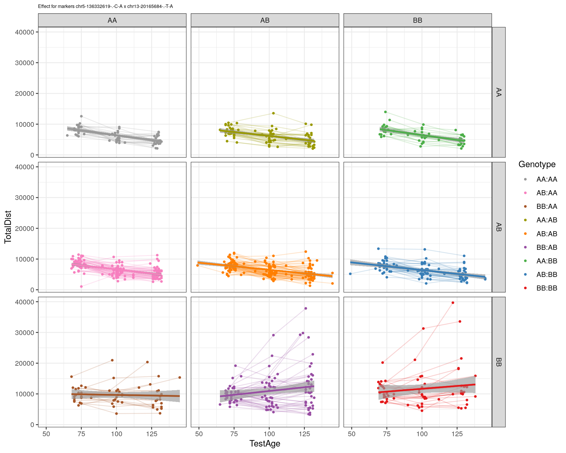
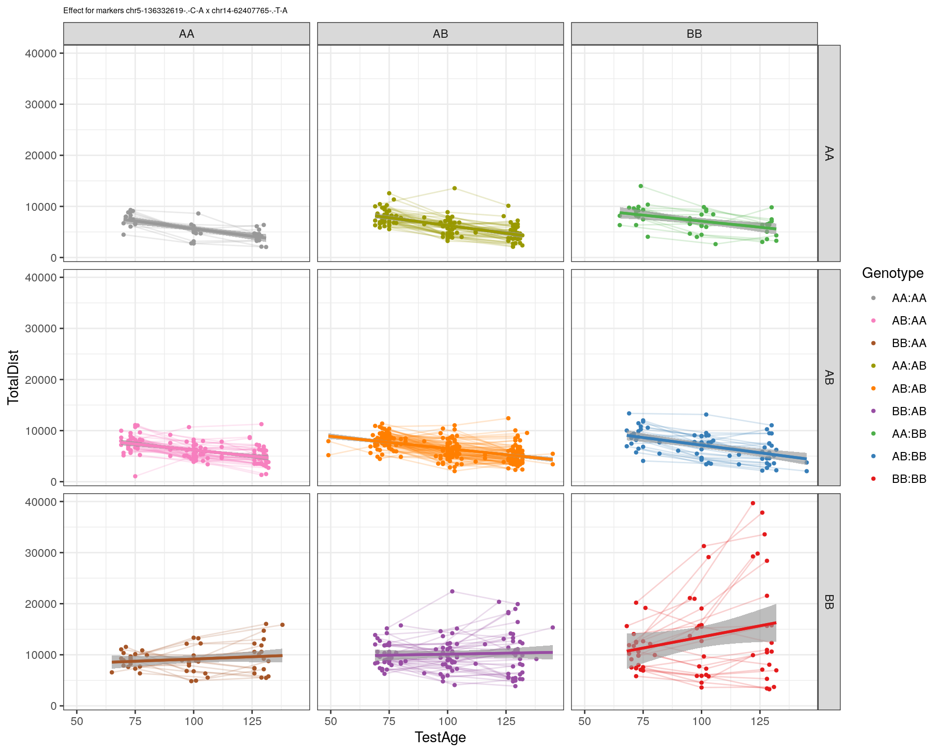
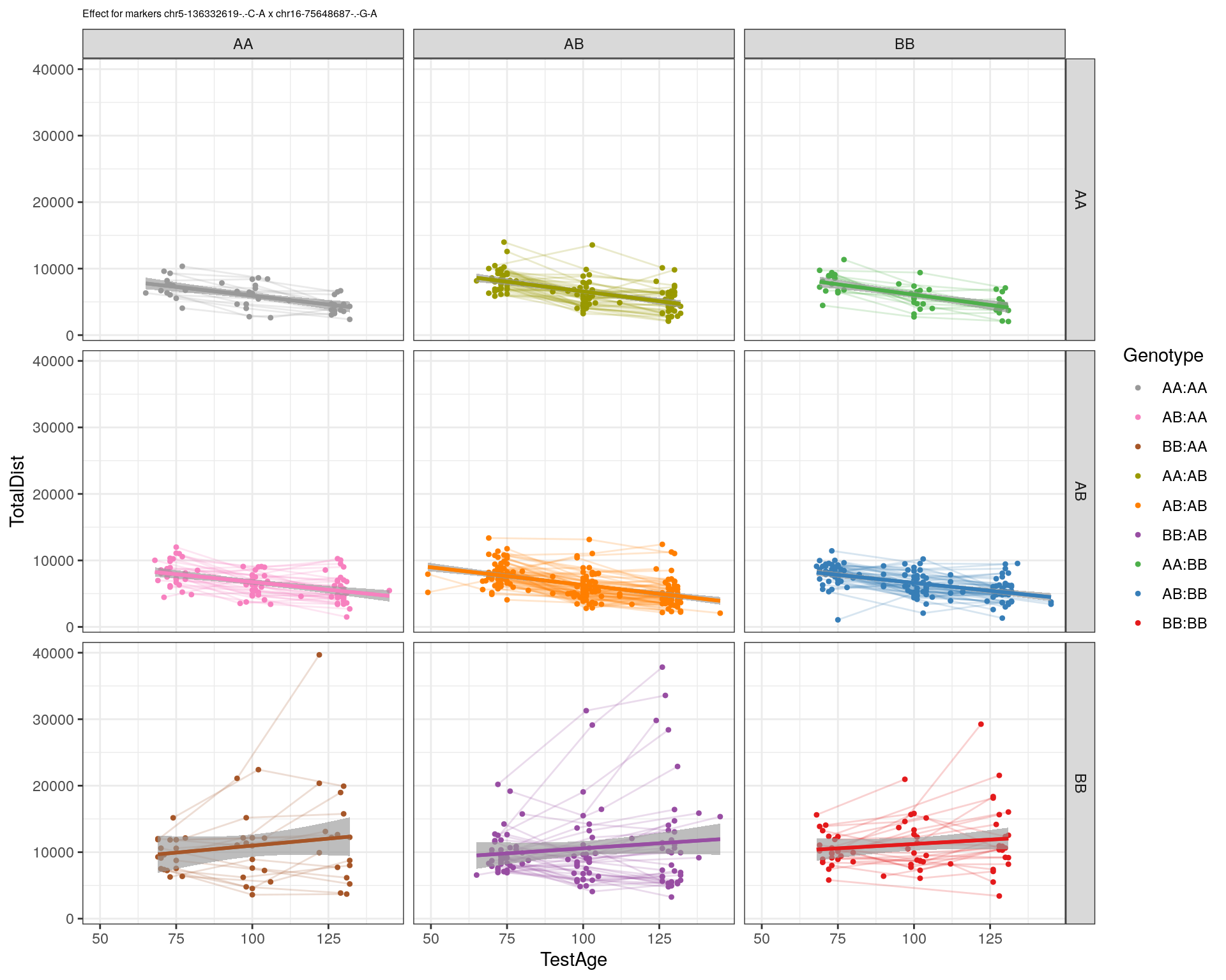
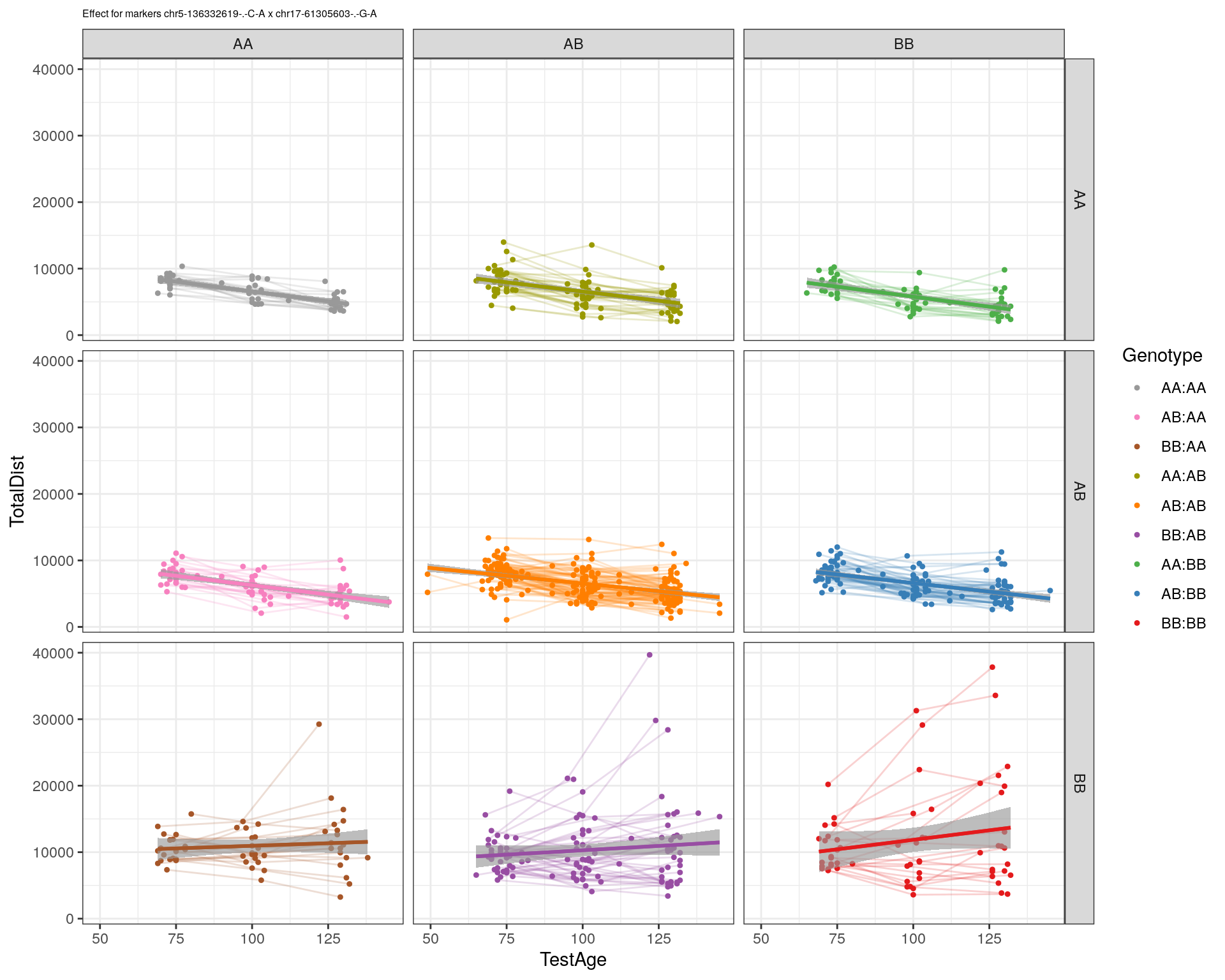
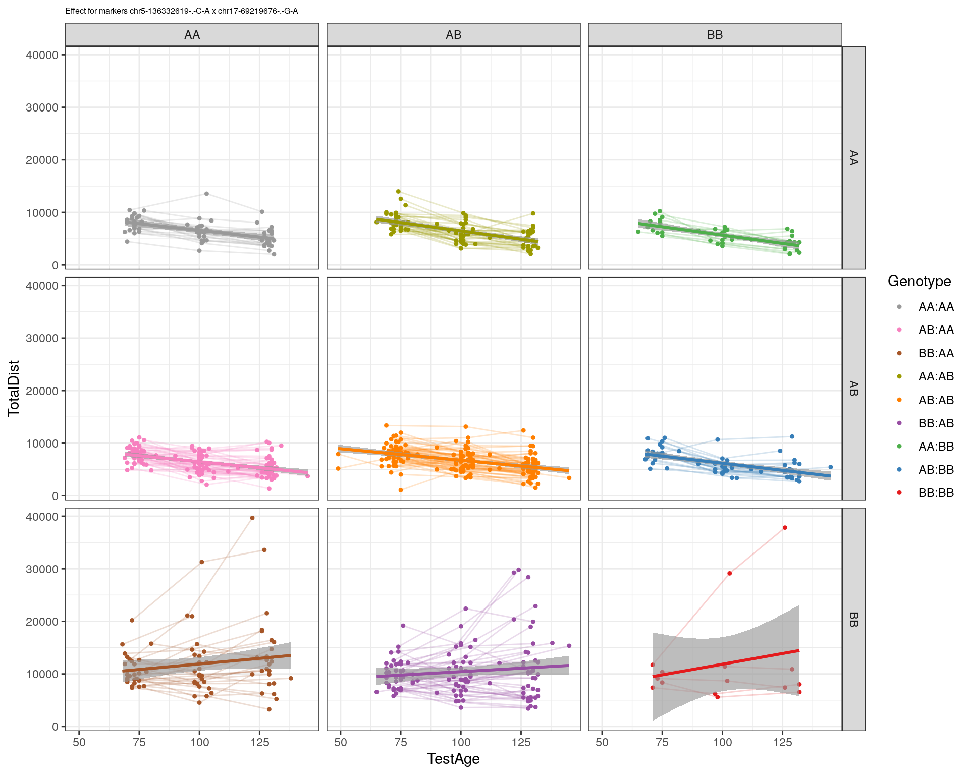
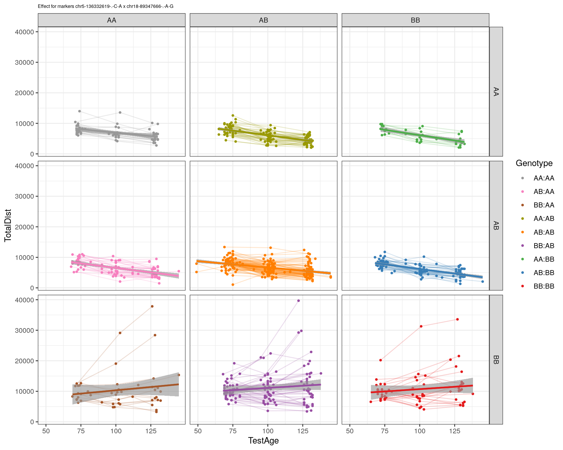
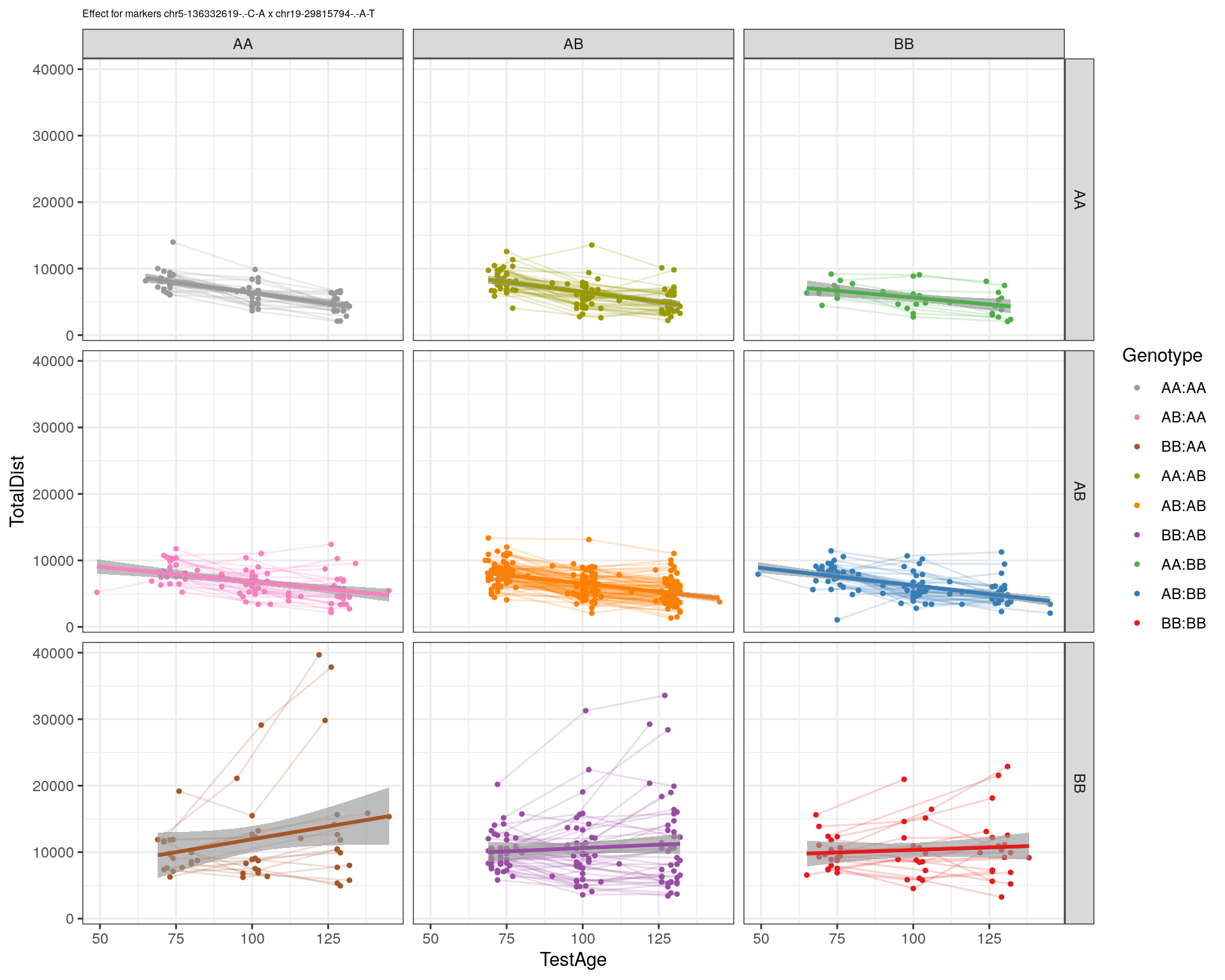
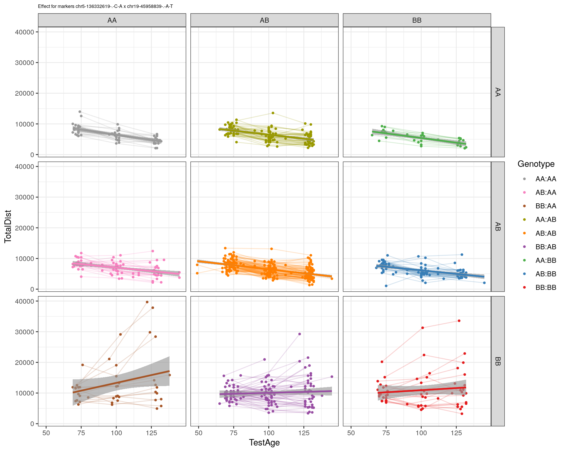
    p2 <- ggplot(subplot, aes(Age, Dist, color=interactions, group=interactions)) +
      geom_point(shape = 20) +
      geom_line(aes(group = AnimalName, color = interactions), show.legend = FALSE, alpha = 0.2) +  
      geom_smooth(method='lm', formula= y~x, show.legend = FALSE) +
      #scale_color_discrete("Genotype") +
      labs(color = "Genotype") +
      ylab("TotalDist") +
      xlab("TestAge") +
      #scale_color_brewer(palette = "Set1") + 
      scale_color_manual(breaks = c("AA:AA", "AB:AA", "BB:AA", "AA:AB",
                                    "AB:AB", "BB:AB", "AA:BB", "AB:BB", "BB:BB"),
                                         #values = RColorBrewer::brewer.pal(9, "Set1")[9:1]) +
                       values = c("#999999", "#F781BF", "#A65628","#9a9a00", "#FF7F00", "#984EA3", "#4DAF4A", "#377EB8", "#E41A1C")) +
      stat_smooth(method="lm", show.legend = FALSE, formula = y~x) + 
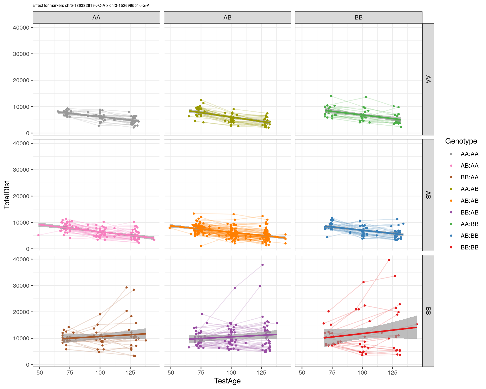
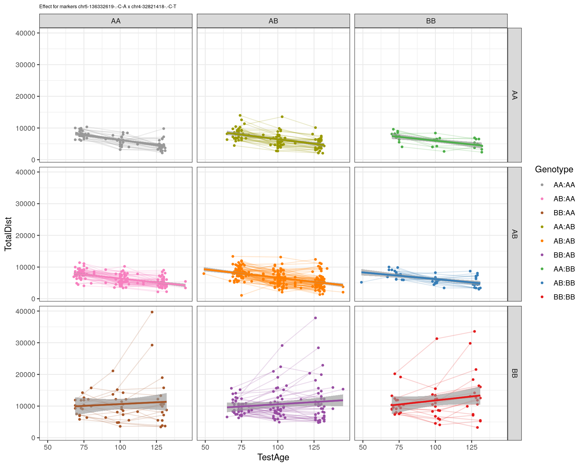
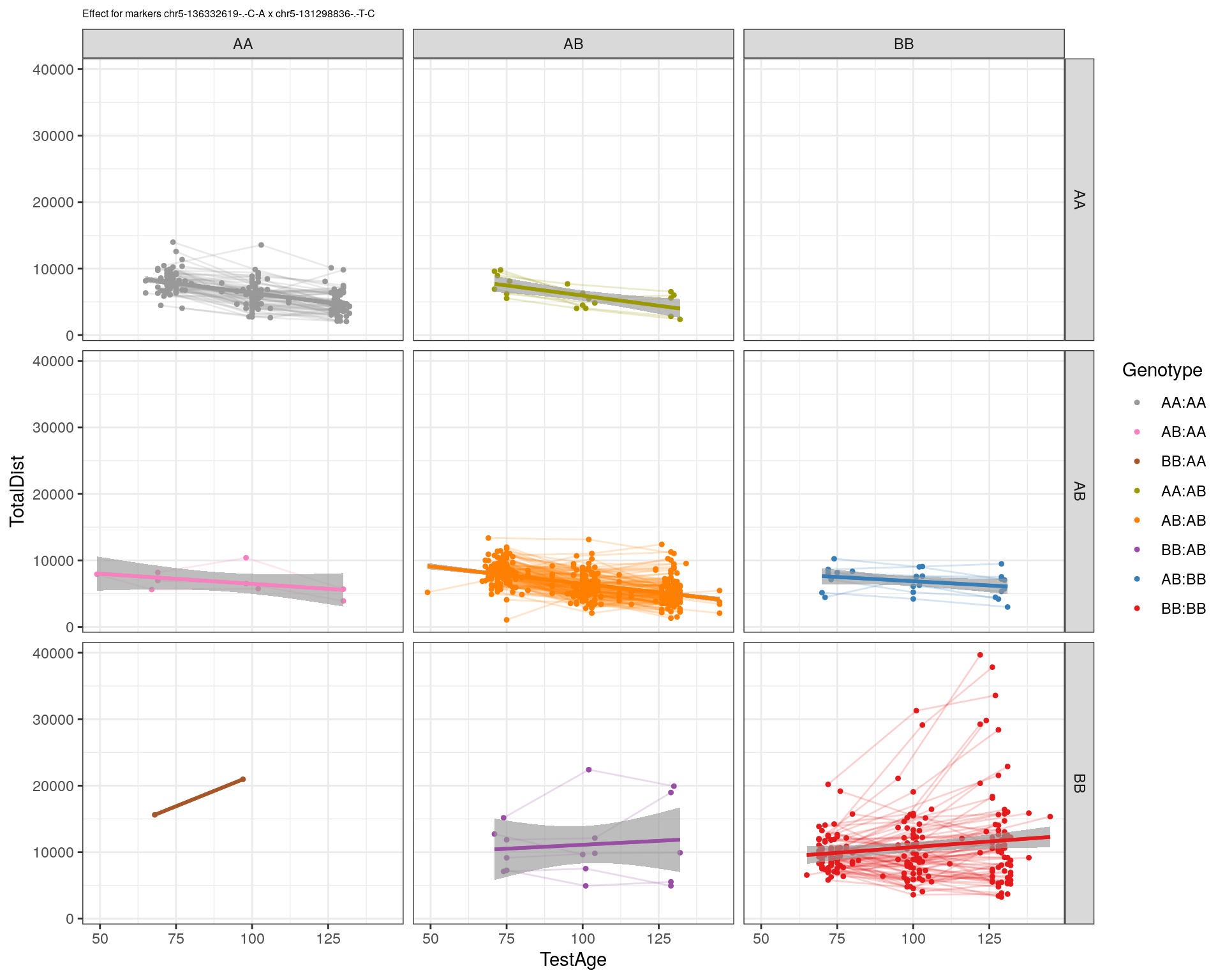
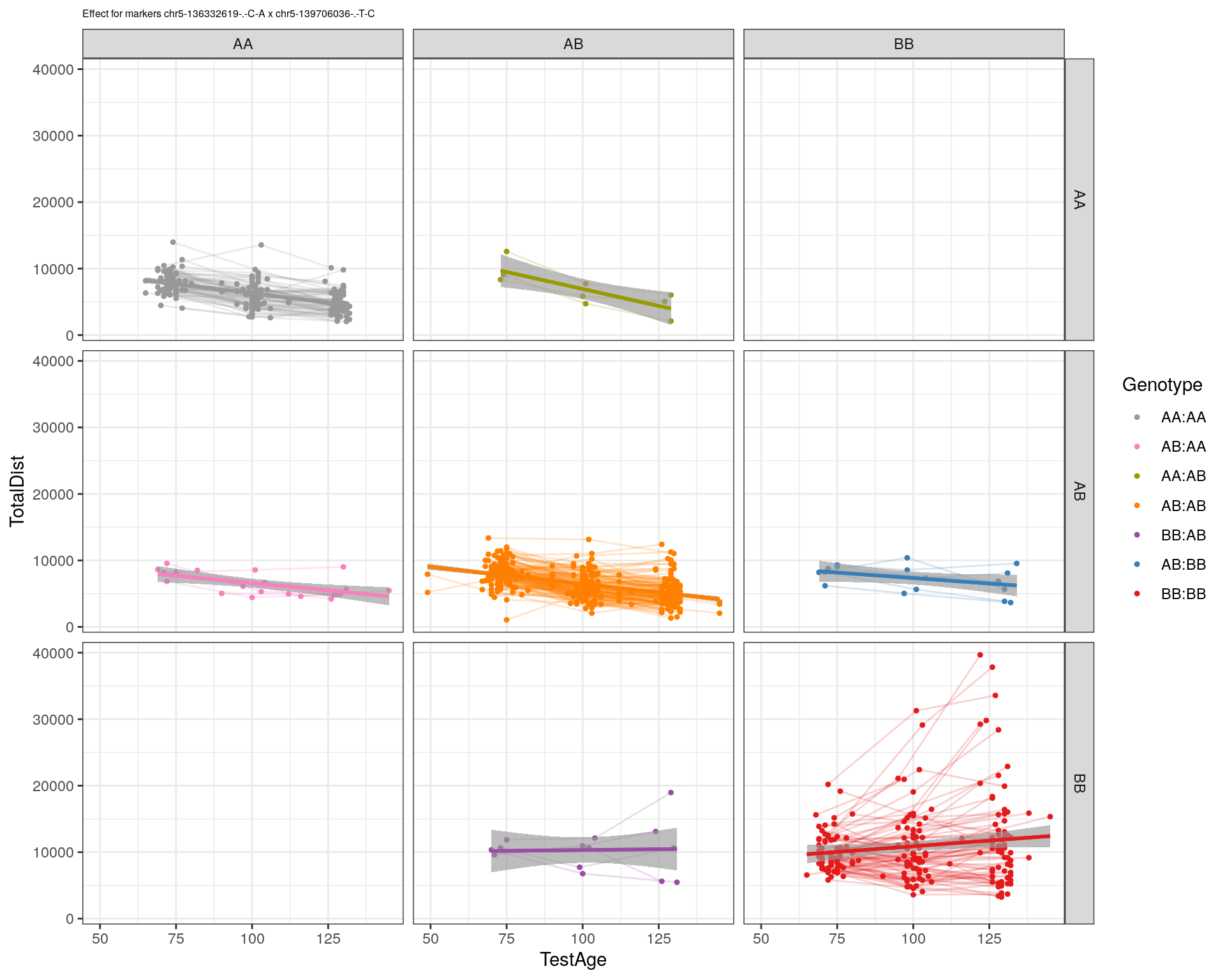
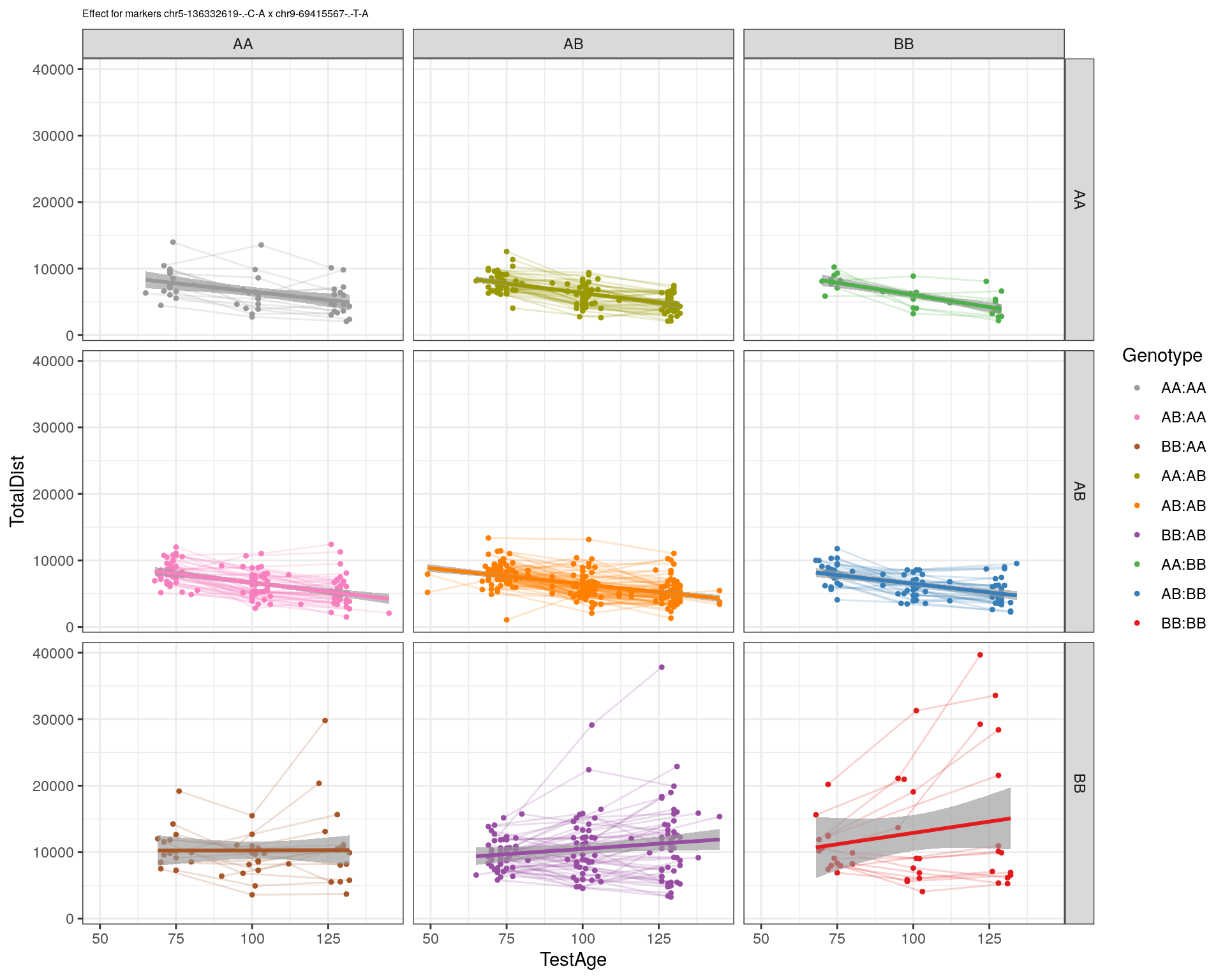
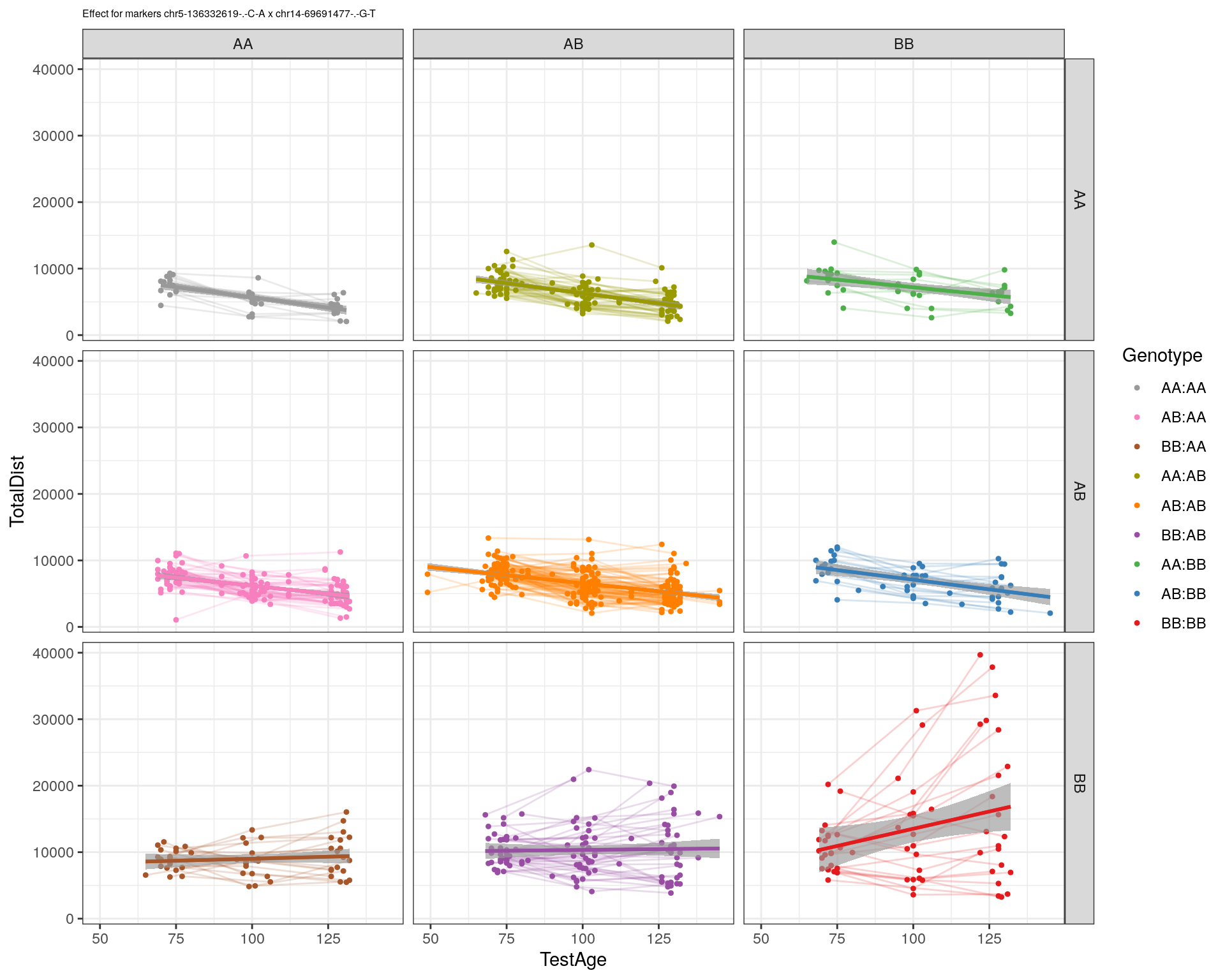
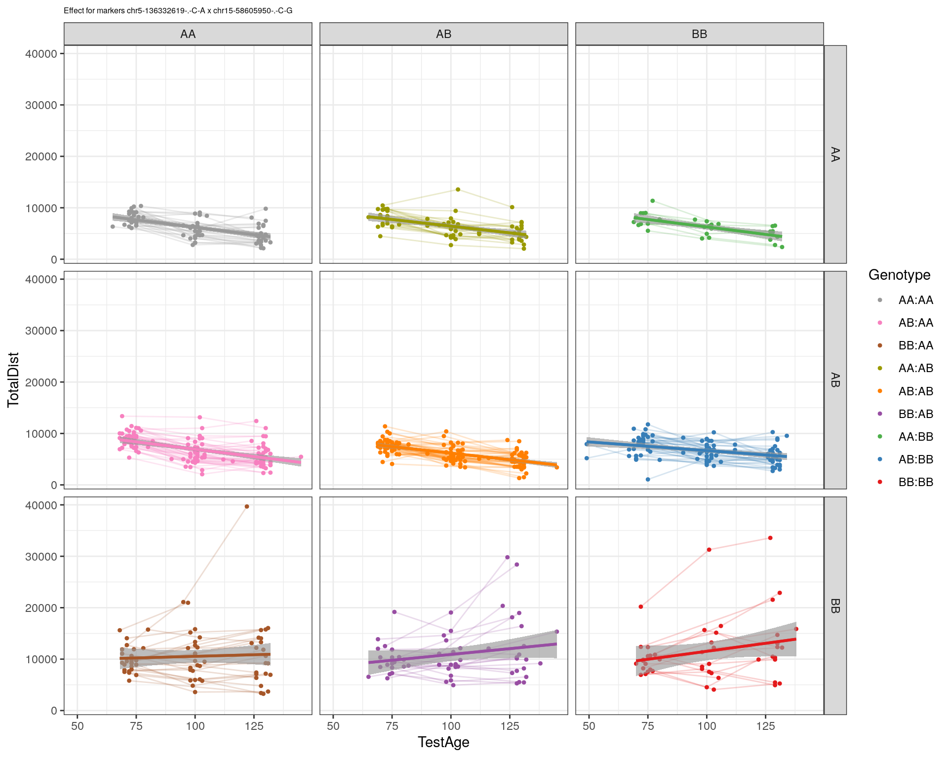
      labs(title=paste0("Effect for markers ", basem, " x ", mar)) +
      facet_grid(subplot[, basem] ~ subplot[, mar]) +
      theme_bw() +
      theme(plot.title = element_text(size=6))
    print(p2)
  }
  #dev.off()
}
plot_graph(WT144, "WT144_effect_for_marker_plots")

png 
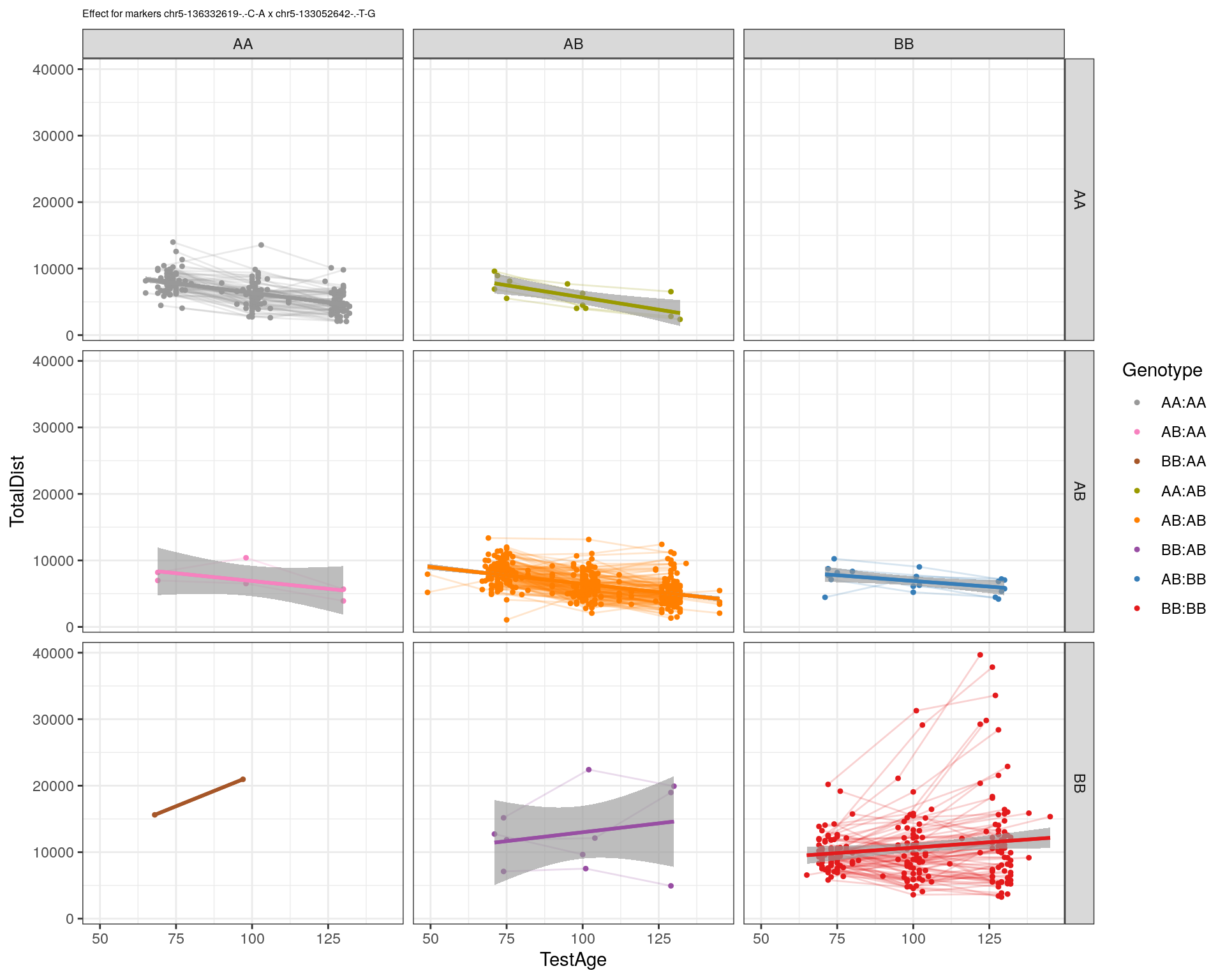
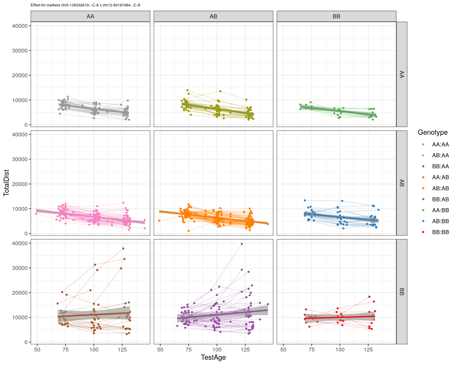
  2 

plot_int_graph(WT144, paste0("WT144_effect_for_marker_", "_int_chr5-136332619-.-C-A"), "chr5-136332619-.-C-A")

[1] "chr1-65643621-.-C-A"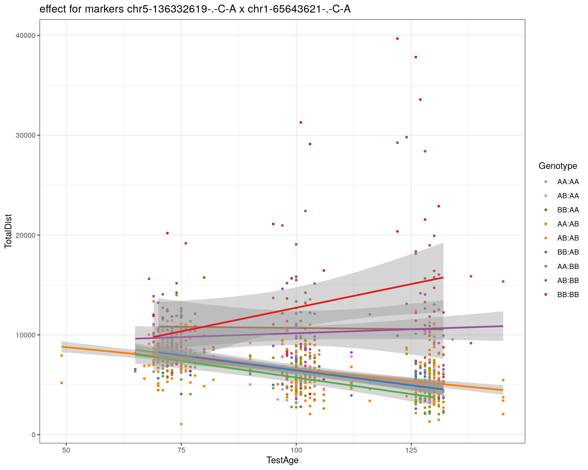

Past versions of “Plot the Dist_vs_age separate by genotype for each marker-1.png”

Version	Author	Date
2470aab	xhyuo	2022-12-24

Past versions of “Plot the Dist_vs_age separate by genotype for each marker-2.png”

Version	Author	Date
2470aab	xhyuo	2022-12-24

[1] "chr1-74679418-.-A-G"

Past versions of “Plot the Dist_vs_age separate by genotype for each marker-3.png”

Version	Author	Date
2470aab	xhyuo	2022-12-24

Past versions of “Plot the Dist_vs_age separate by genotype for each marker-4.png”

Version	Author	Date
2470aab	xhyuo	2022-12-24

[1] "chr1-79823528-.-A-G"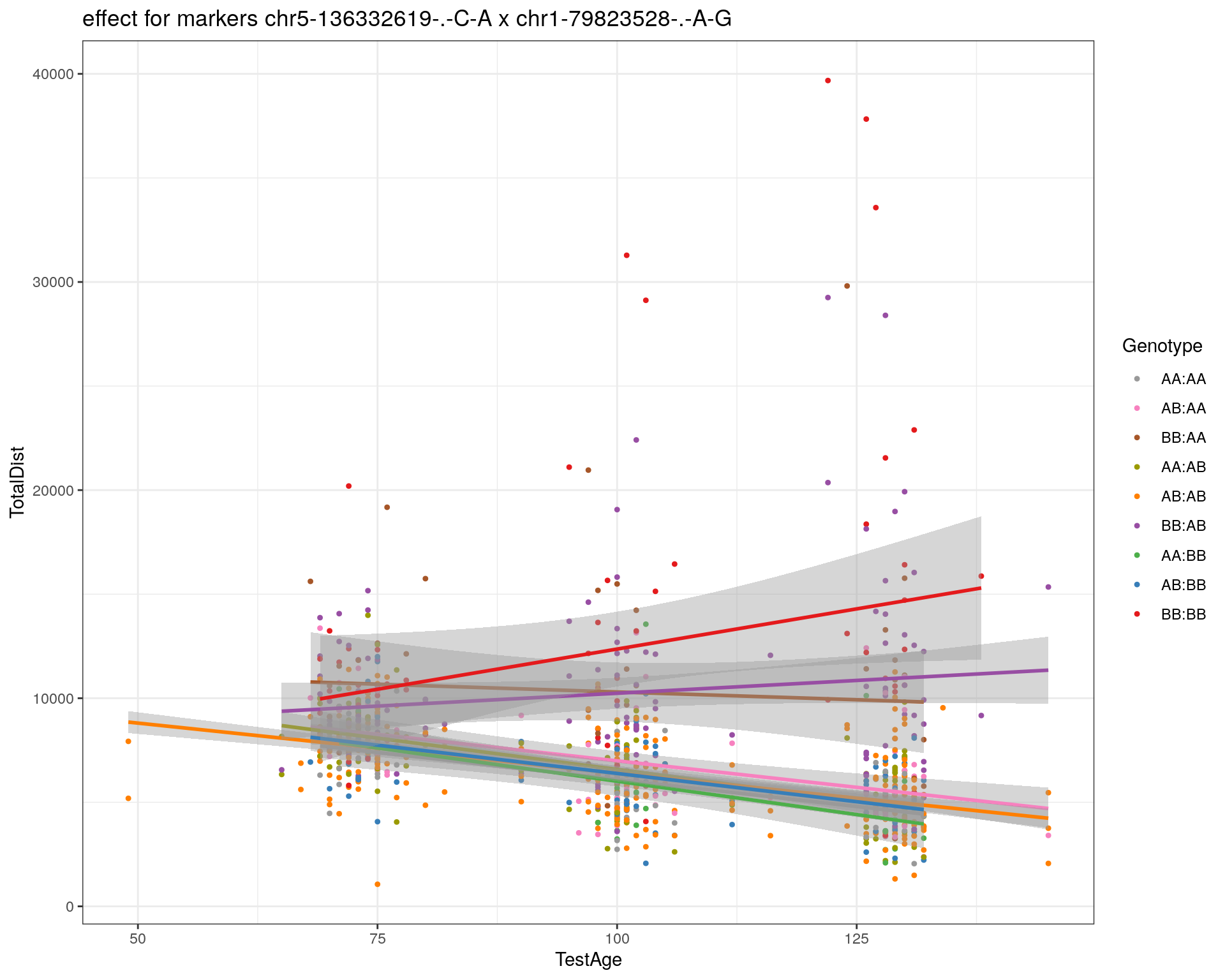

Past versions of “Plot the Dist_vs_age separate by genotype for each marker-5.png”

Version	Author	Date
2470aab	xhyuo	2022-12-24

Past versions of “Plot the Dist_vs_age separate by genotype for each marker-6.png”

Version	Author	Date
2470aab	xhyuo	2022-12-24

[1] "chr1-86851039-.-A-G"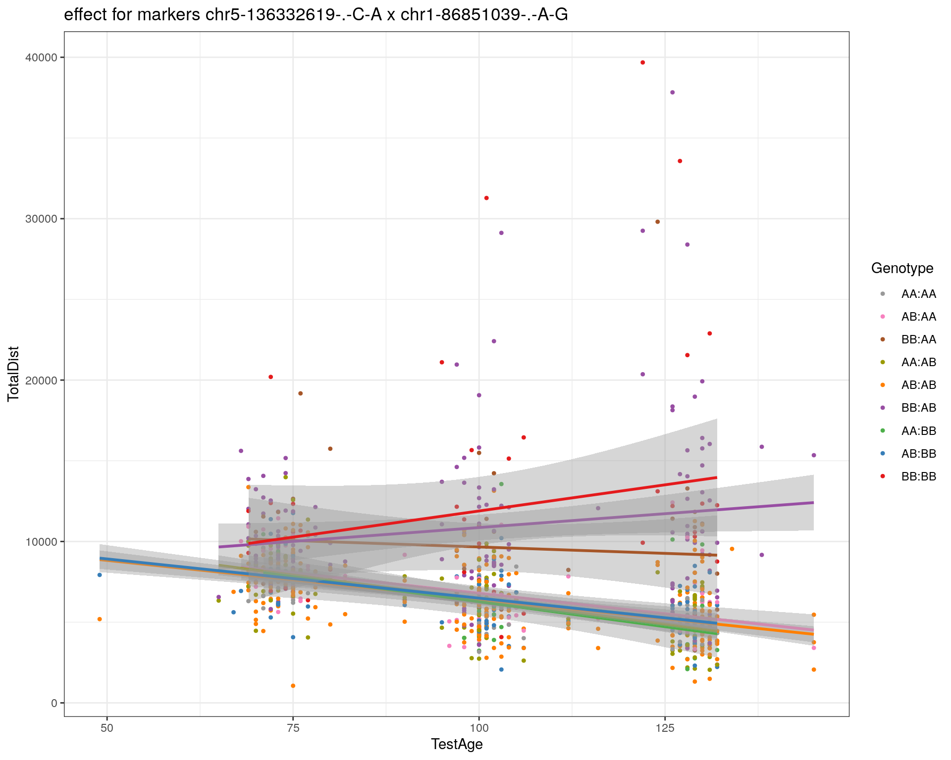

Past versions of “Plot the Dist_vs_age separate by genotype for each marker-7.png”

Version	Author	Date
2470aab	xhyuo	2022-12-24

Past versions of “Plot the Dist_vs_age separate by genotype for each marker-8.png”

Version	Author	Date
2470aab	xhyuo	2022-12-24

[1] "chr1-188155143-.-G-A"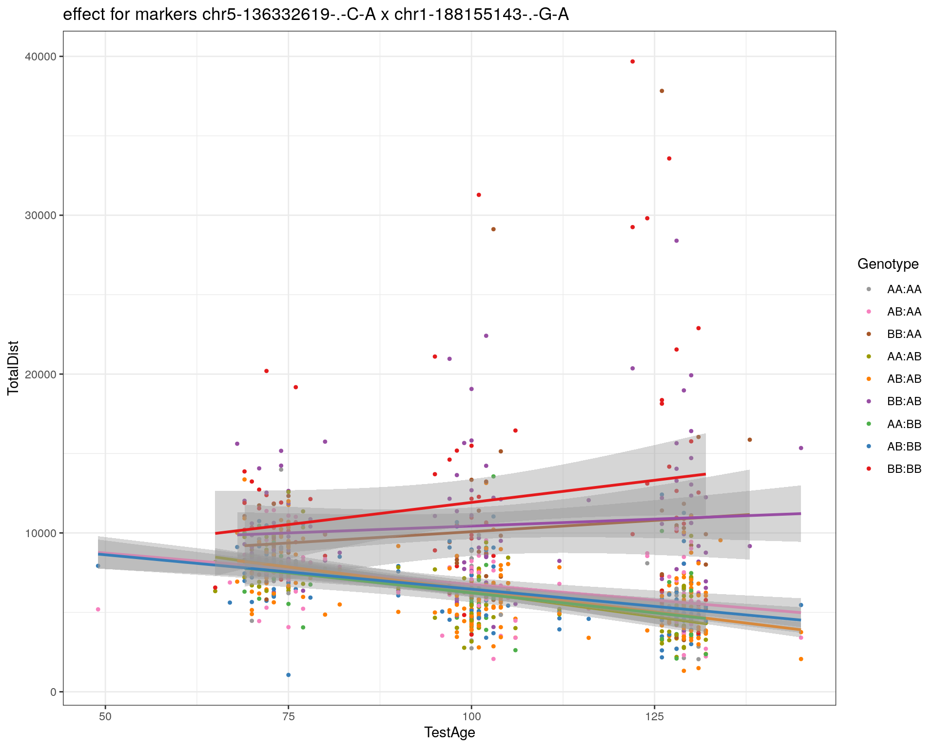

Past versions of “Plot the Dist_vs_age separate by genotype for each marker-9.png”

Version	Author	Date
2470aab	xhyuo	2022-12-24

Past versions of “Plot the Dist_vs_age separate by genotype for each marker-10.png”

Version	Author	Date
2470aab	xhyuo	2022-12-24

[1] "chr2-7018694-.-G-T"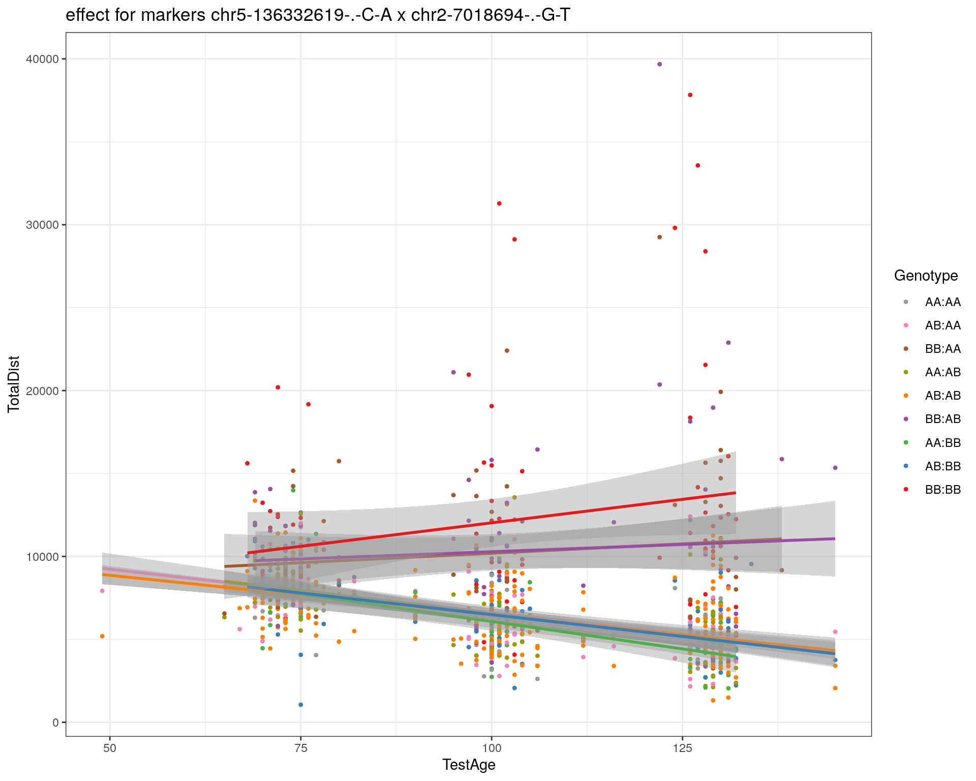

Past versions of “Plot the Dist_vs_age separate by genotype for each marker-11.png”

Version	Author	Date
2470aab	xhyuo	2022-12-24

Past versions of “Plot the Dist_vs_age separate by genotype for each marker-12.png”

Version	Author	Date
2470aab	xhyuo	2022-12-24

[1] "chr2-79706301-.-T-A"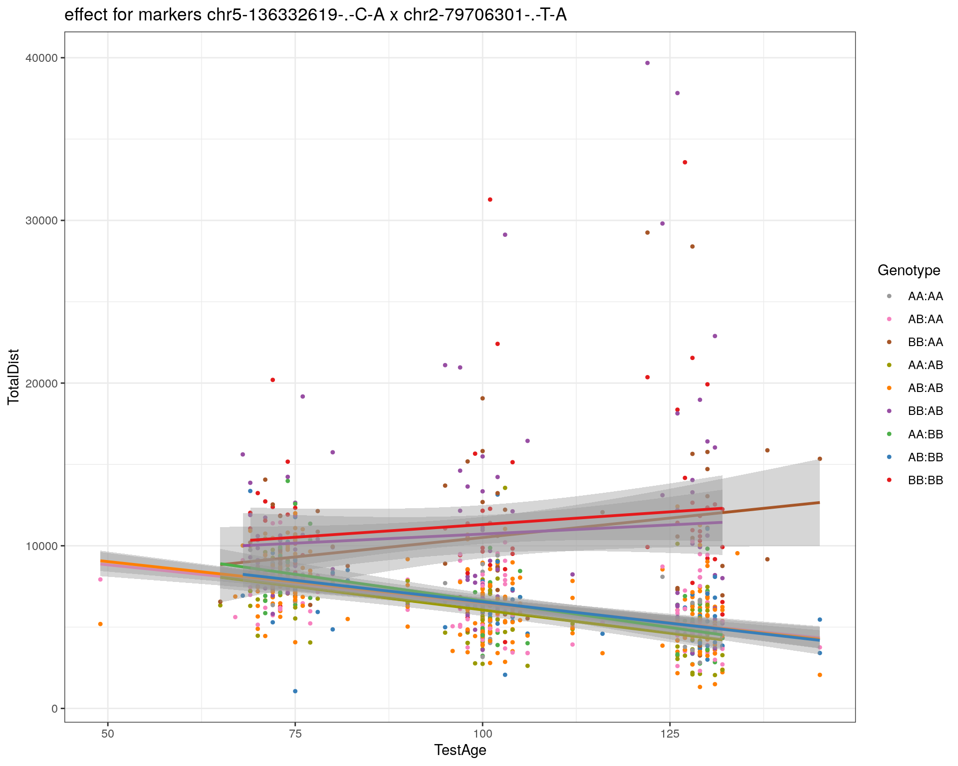

Past versions of “Plot the Dist_vs_age separate by genotype for each marker-13.png”

Version	Author	Date
2470aab	xhyuo	2022-12-24

Past versions of “Plot the Dist_vs_age separate by genotype for each marker-14.png”

Version	Author	Date
2470aab	xhyuo	2022-12-24

[1] "chr2-92367783-.-T-C"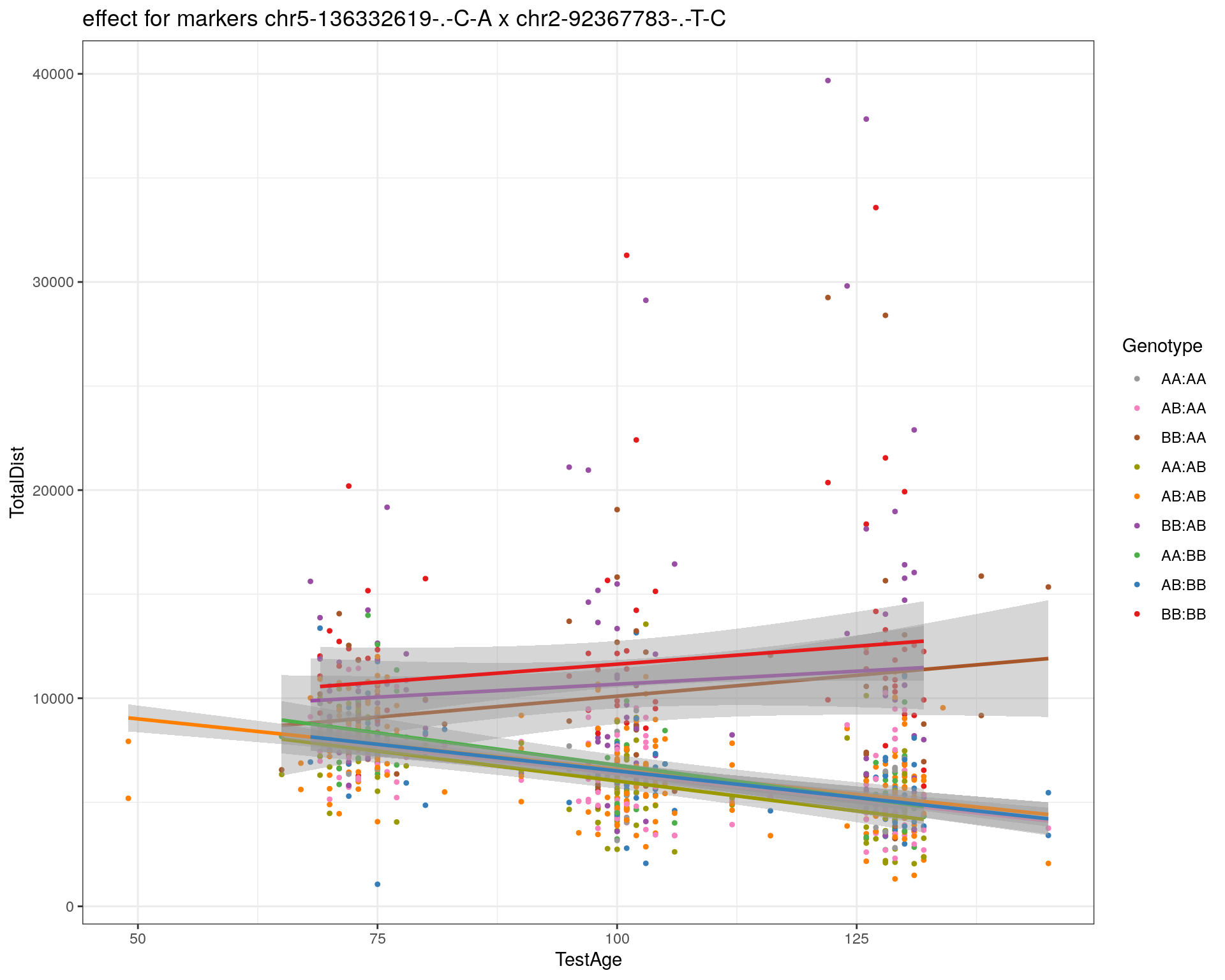

Past versions of “Plot the Dist_vs_age separate by genotype for each marker-15.png”

Version	Author	Date
2470aab	xhyuo	2022-12-24

Past versions of “Plot the Dist_vs_age separate by genotype for each marker-16.png”

Version	Author	Date
2470aab	xhyuo	2022-12-24

[1] "chr2-95118744-.-T-A"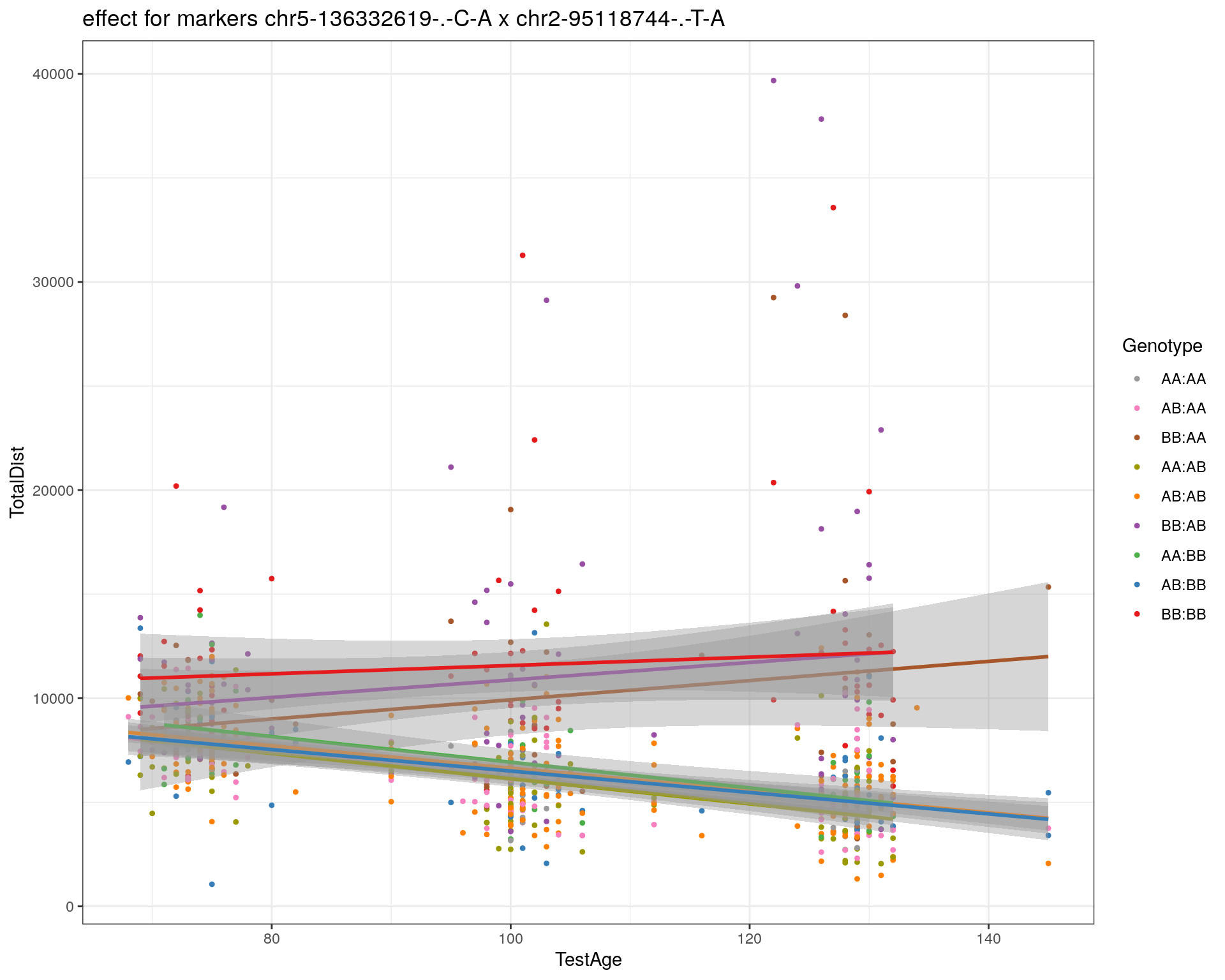

Past versions of “Plot the Dist_vs_age separate by genotype for each marker-17.png”

Version	Author	Date
2470aab	xhyuo	2022-12-24

Past versions of “Plot the Dist_vs_age separate by genotype for each marker-18.png”

Version	Author	Date
2470aab	xhyuo	2022-12-24

[1] "chr2-102169266-.-C-T"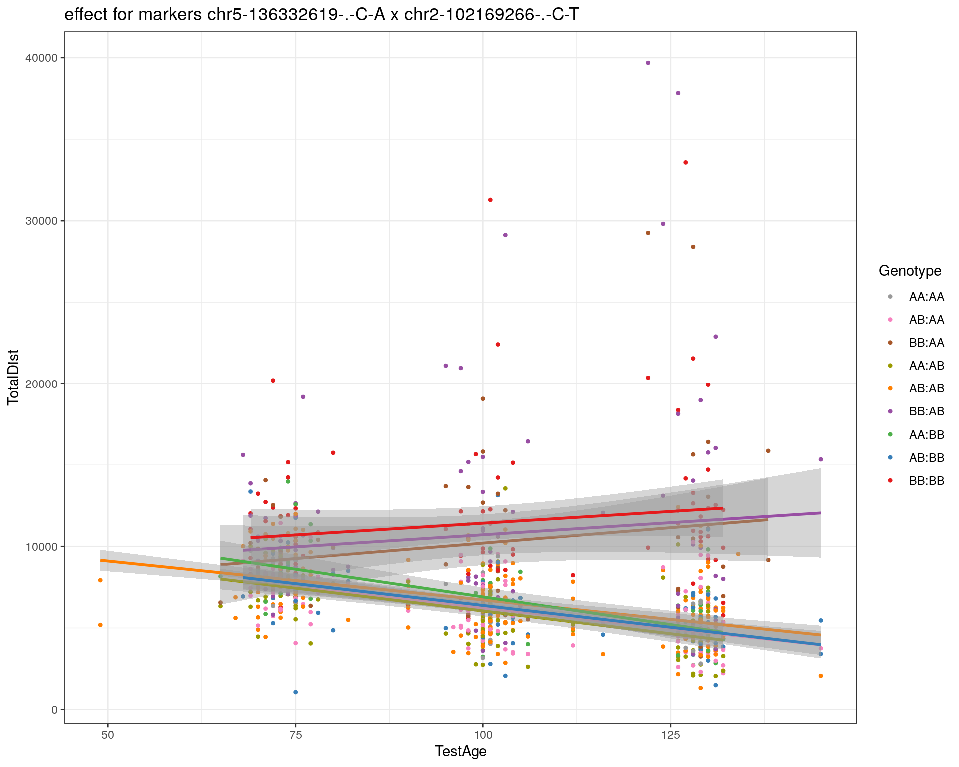

Past versions of “Plot the Dist_vs_age separate by genotype for each marker-19.png”

Version	Author	Date
2470aab	xhyuo	2022-12-24

Past versions of “Plot the Dist_vs_age separate by genotype for each marker-20.png”

Version	Author	Date
2470aab	xhyuo	2022-12-24

[1] "chr2-130405980-.-A-T"

Past versions of “Plot the Dist_vs_age separate by genotype for each marker-21.png”

Version	Author	Date
2470aab	xhyuo	2022-12-24

Past versions of “Plot the Dist_vs_age separate by genotype for each marker-22.png”

Version	Author	Date
2470aab	xhyuo	2022-12-24

[1] "chr2-137498061-.-T-A"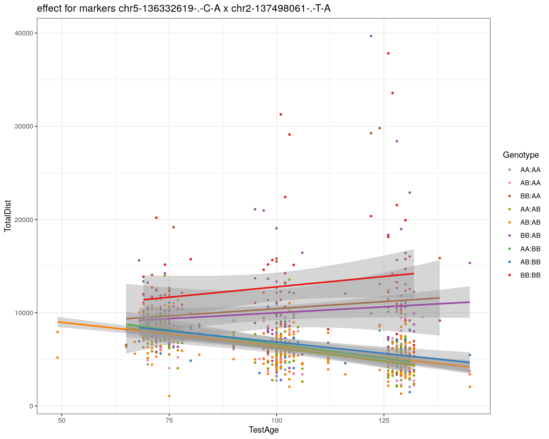

Past versions of “Plot the Dist_vs_age separate by genotype for each marker-23.png”

Version	Author	Date
2470aab	xhyuo	2022-12-24

Past versions of “Plot the Dist_vs_age separate by genotype for each marker-24.png”

Version	Author	Date
2470aab	xhyuo	2022-12-24

[1] "chr2-145128463-.-A-T"

Past versions of “Plot the Dist_vs_age separate by genotype for each marker-25.png”

Version	Author	Date
2470aab	xhyuo	2022-12-24

Past versions of “Plot the Dist_vs_age separate by genotype for each marker-26.png”

Version	Author	Date
2470aab	xhyuo	2022-12-24

[1] "chr3-59218564-.-T-A"

Past versions of “Plot the Dist_vs_age separate by genotype for each marker-27.png”

Version	Author	Date
2470aab	xhyuo	2022-12-24

Past versions of “Plot the Dist_vs_age separate by genotype for each marker-28.png”

Version	Author	Date
2470aab	xhyuo	2022-12-24

[1] "chr3-98881230-.-G-A"

Past versions of “Plot the Dist_vs_age separate by genotype for each marker-29.png”

Version	Author	Date
2470aab	xhyuo	2022-12-24

Past versions of “Plot the Dist_vs_age separate by genotype for each marker-30.png”

Version	Author	Date
2470aab	xhyuo	2022-12-24

[1] "chr3-106985708-.-A-C"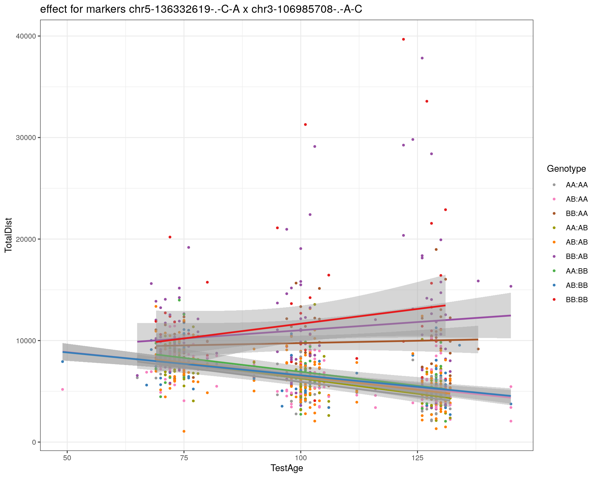

Past versions of “Plot the Dist_vs_age separate by genotype for each marker-31.png”

Version	Author	Date
2470aab	xhyuo	2022-12-24

Past versions of “Plot the Dist_vs_age separate by genotype for each marker-32.png”

Version	Author	Date
2470aab	xhyuo	2022-12-24

[1] "chr3-135614002-.-T-G"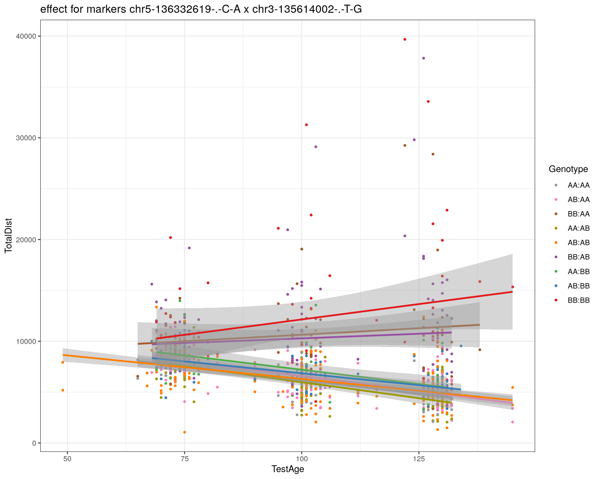

Past versions of “Plot the Dist_vs_age separate by genotype for each marker-33.png”

Version	Author	Date
2470aab	xhyuo	2022-12-24

Past versions of “Plot the Dist_vs_age separate by genotype for each marker-34.png”

Version	Author	Date
2470aab	xhyuo	2022-12-24

[1] "chr3-145286160-.-C-A"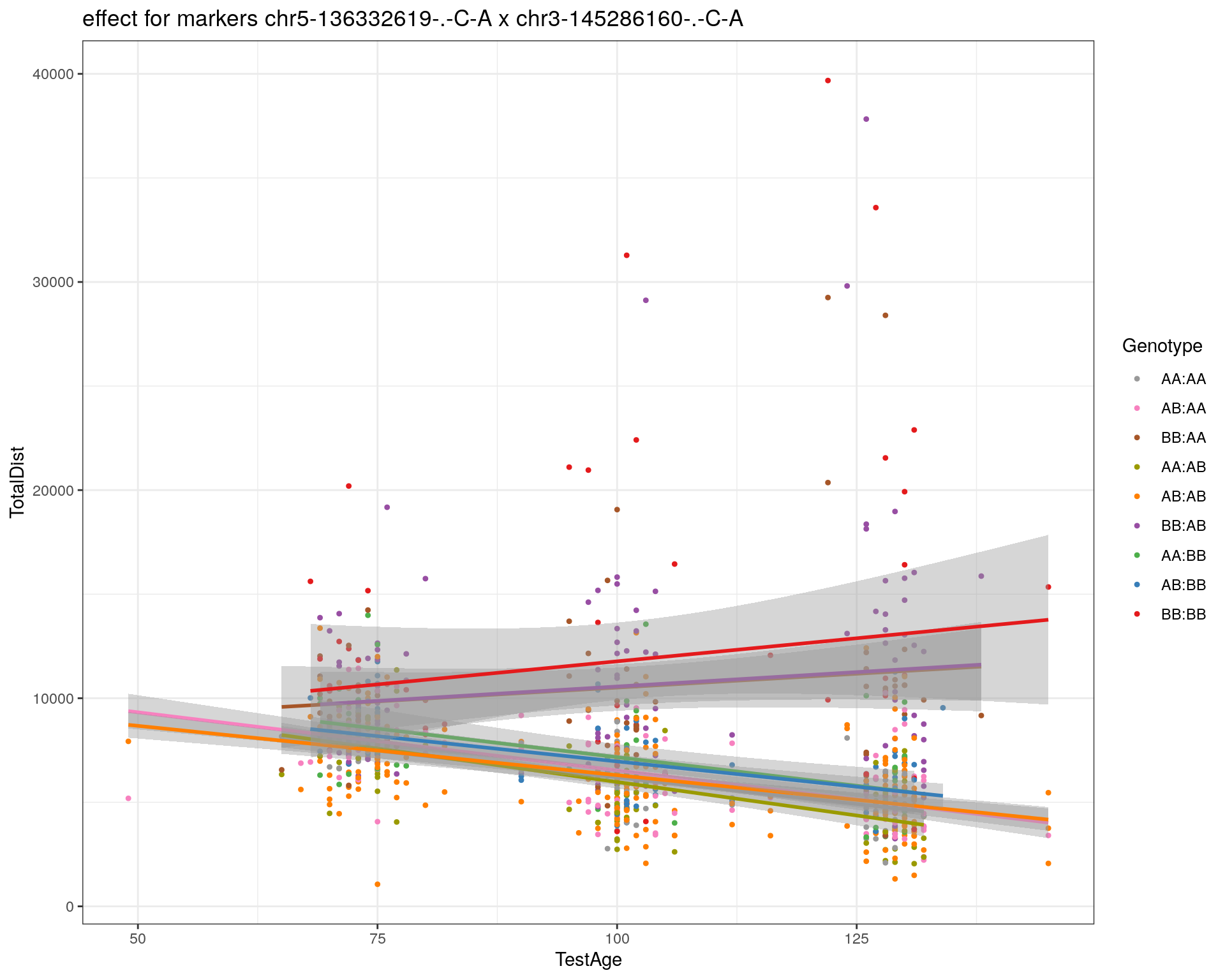

Past versions of “Plot the Dist_vs_age separate by genotype for each marker-35.png”

Version	Author	Date
2470aab	xhyuo	2022-12-24

Past versions of “Plot the Dist_vs_age separate by genotype for each marker-36.png”

Version	Author	Date
2470aab	xhyuo	2022-12-24

[1] "chr3-146750531-.-A-G"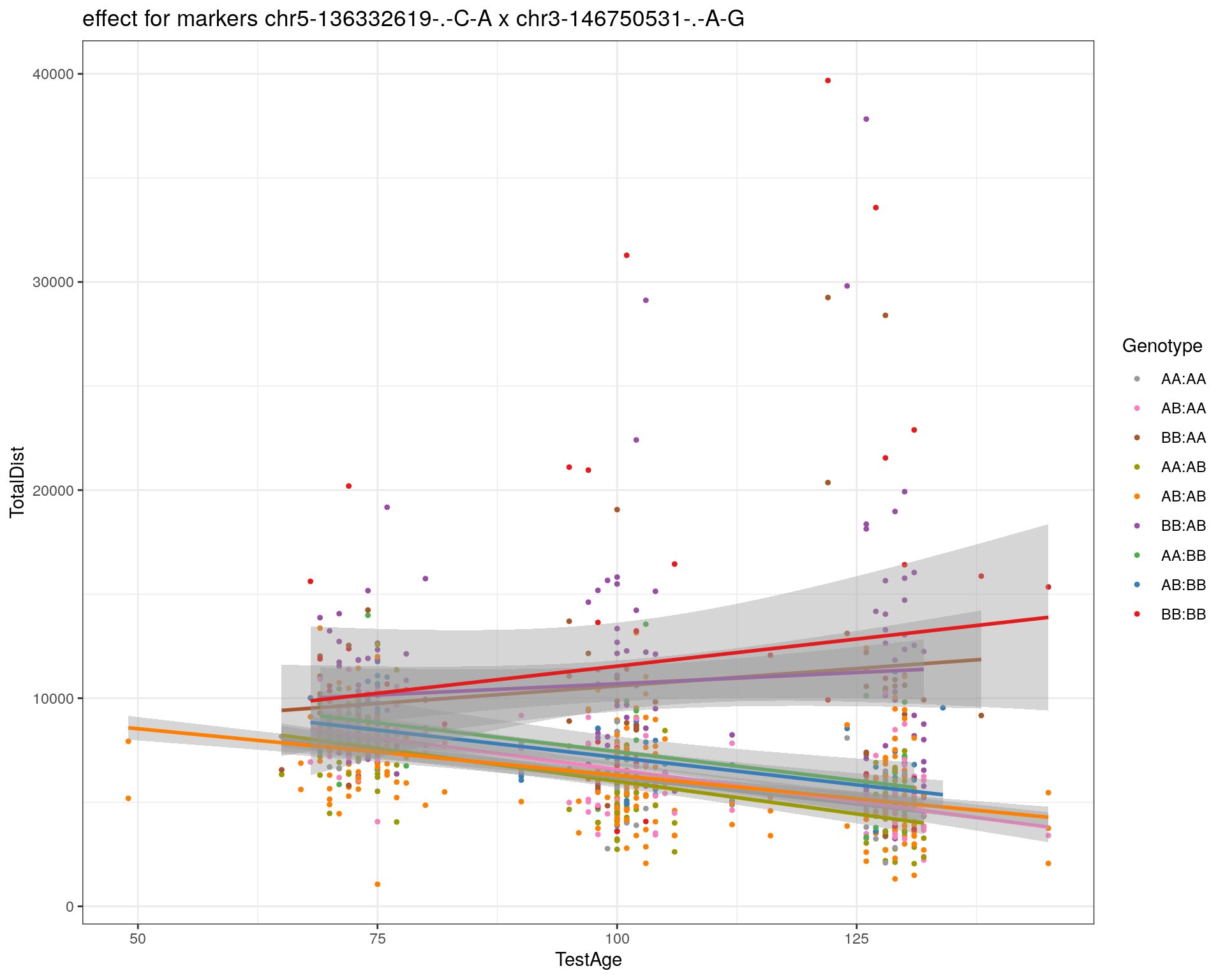

Past versions of “Plot the Dist_vs_age separate by genotype for each marker-37.png”

Version	Author	Date
2470aab	xhyuo	2022-12-24

Past versions of “Plot the Dist_vs_age separate by genotype for each marker-38.png”

Version	Author	Date
2470aab	xhyuo	2022-12-24

[1] "chr3-152699551-.-G-A"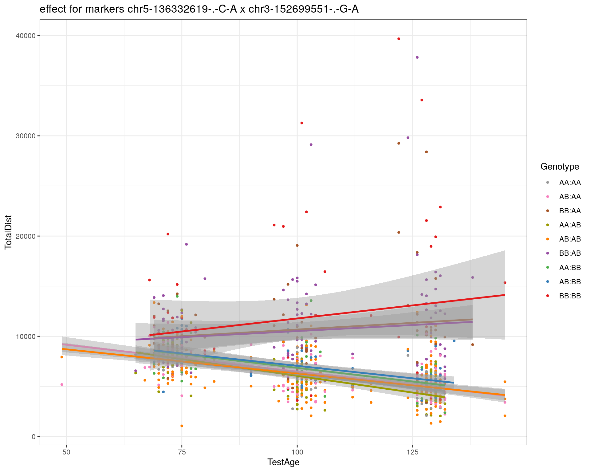

Past versions of “Plot the Dist_vs_age separate by genotype for each marker-39.png”

Version	Author	Date
2470aab	xhyuo	2022-12-24

Past versions of “Plot the Dist_vs_age separate by genotype for each marker-40.png”

Version	Author	Date
2470aab	xhyuo	2022-12-24

[1] "chr4-32821418-.-C-T"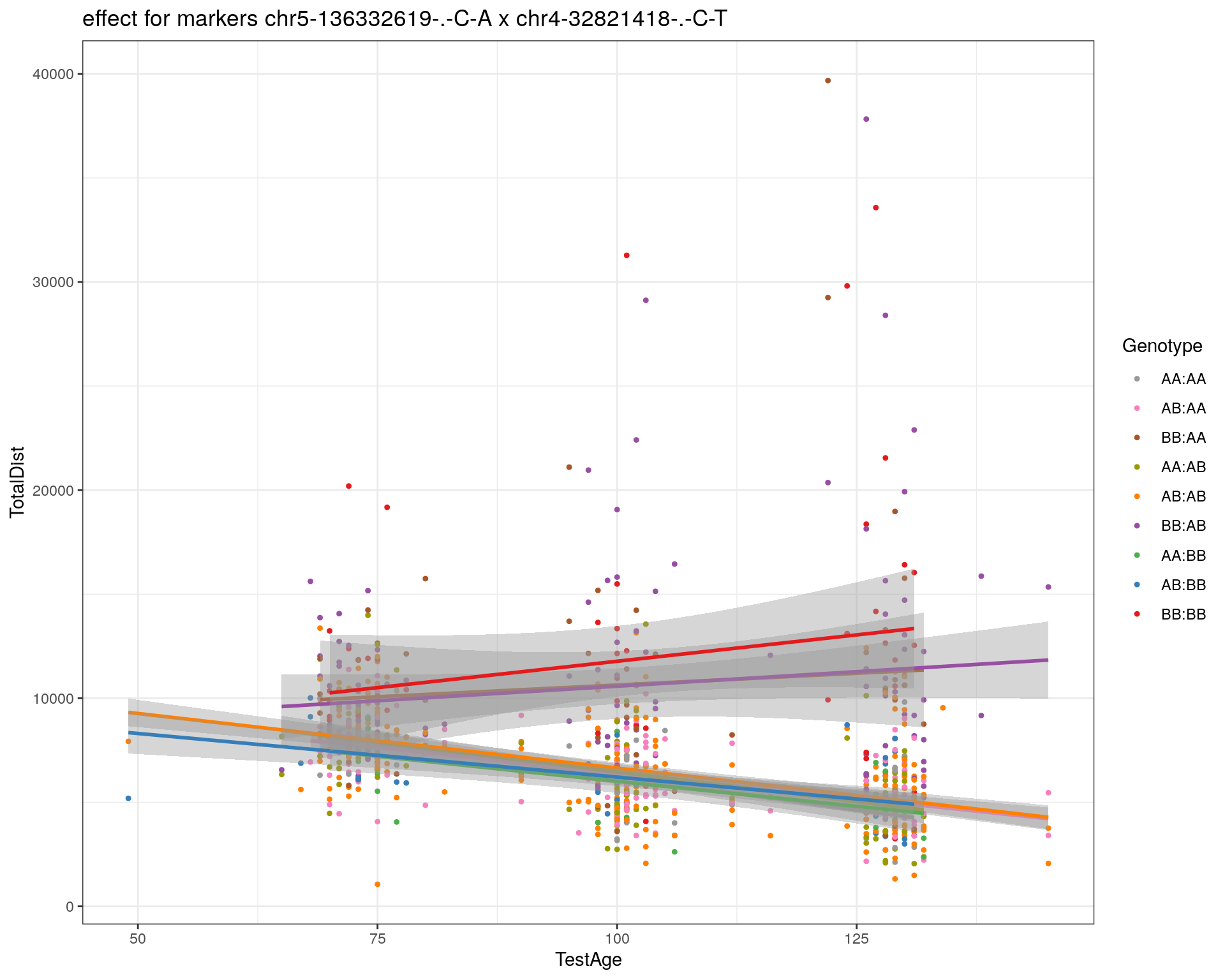

Past versions of “Plot the Dist_vs_age separate by genotype for each marker-41.png”

Version	Author	Date
2470aab	xhyuo	2022-12-24

Past versions of “Plot the Dist_vs_age separate by genotype for each marker-42.png”

Version	Author	Date
2470aab	xhyuo	2022-12-24

[1] "chr5-75264187-.-T-C"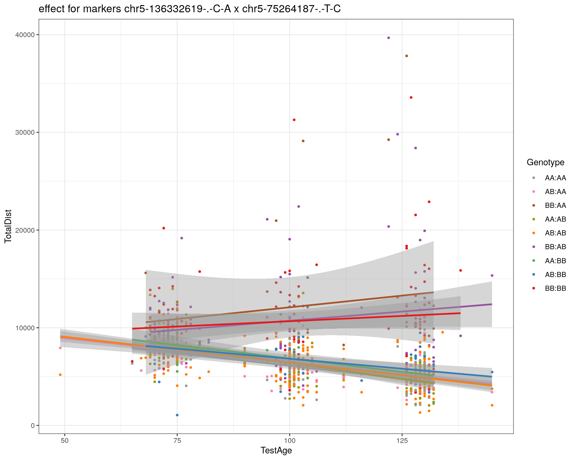

Past versions of “Plot the Dist_vs_age separate by genotype for each marker-43.png”

Version	Author	Date
2470aab	xhyuo	2022-12-24

Past versions of “Plot the Dist_vs_age separate by genotype for each marker-44.png”

Version	Author	Date
2470aab	xhyuo	2022-12-24

[1] "chr5-90233933-.-A-T"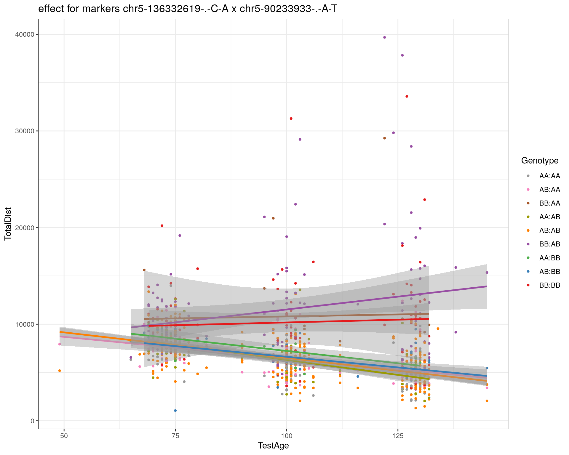

Past versions of “Plot the Dist_vs_age separate by genotype for each marker-45.png”

Version	Author	Date
2470aab	xhyuo	2022-12-24

Past versions of “Plot the Dist_vs_age separate by genotype for each marker-46.png”

Version	Author	Date
2470aab	xhyuo	2022-12-24

[1] "chr5-97607237-.-T-A"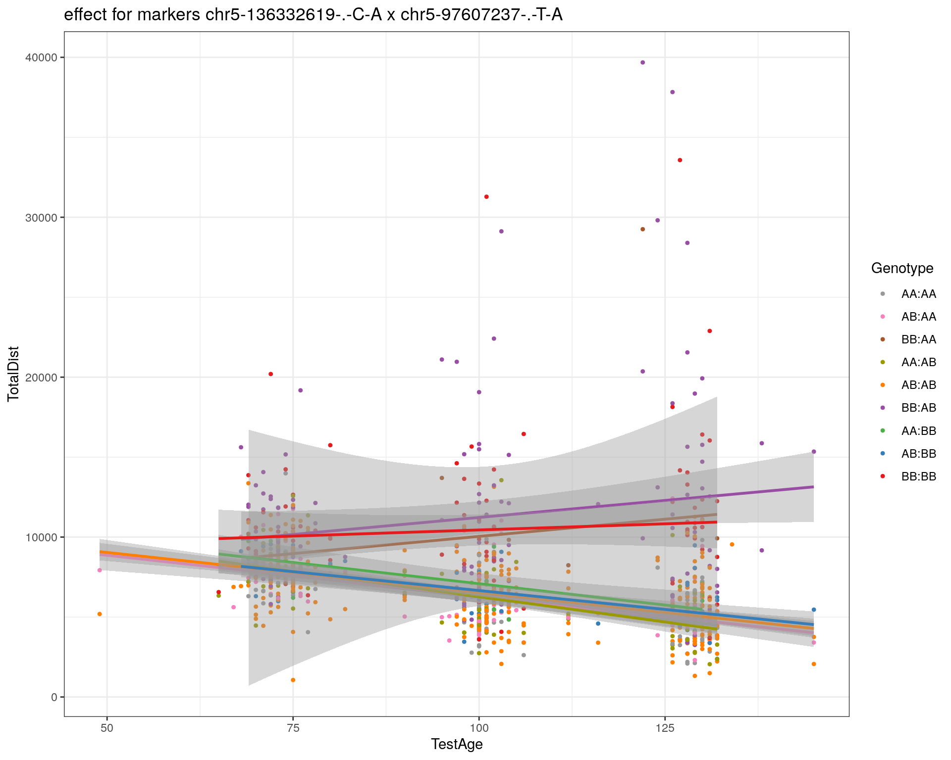

Past versions of “Plot the Dist_vs_age separate by genotype for each marker-47.png”

Version	Author	Date
2470aab	xhyuo	2022-12-24

Past versions of “Plot the Dist_vs_age separate by genotype for each marker-48.png”

Version	Author	Date
2470aab	xhyuo	2022-12-24

[1] "chr5-107507008-.-C-T"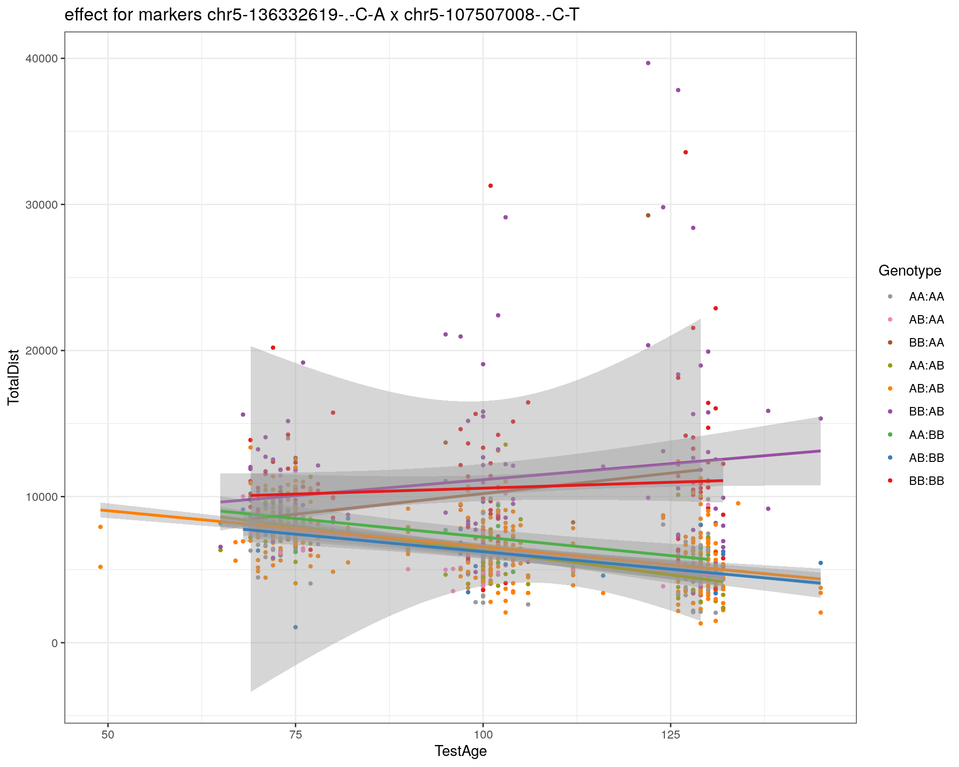

Past versions of “Plot the Dist_vs_age separate by genotype for each marker-49.png”

Version	Author	Date
2470aab	xhyuo	2022-12-24

Past versions of “Plot the Dist_vs_age separate by genotype for each marker-50.png”

Version	Author	Date
2470aab	xhyuo	2022-12-24

[1] "chr5-112799362-.-C-T"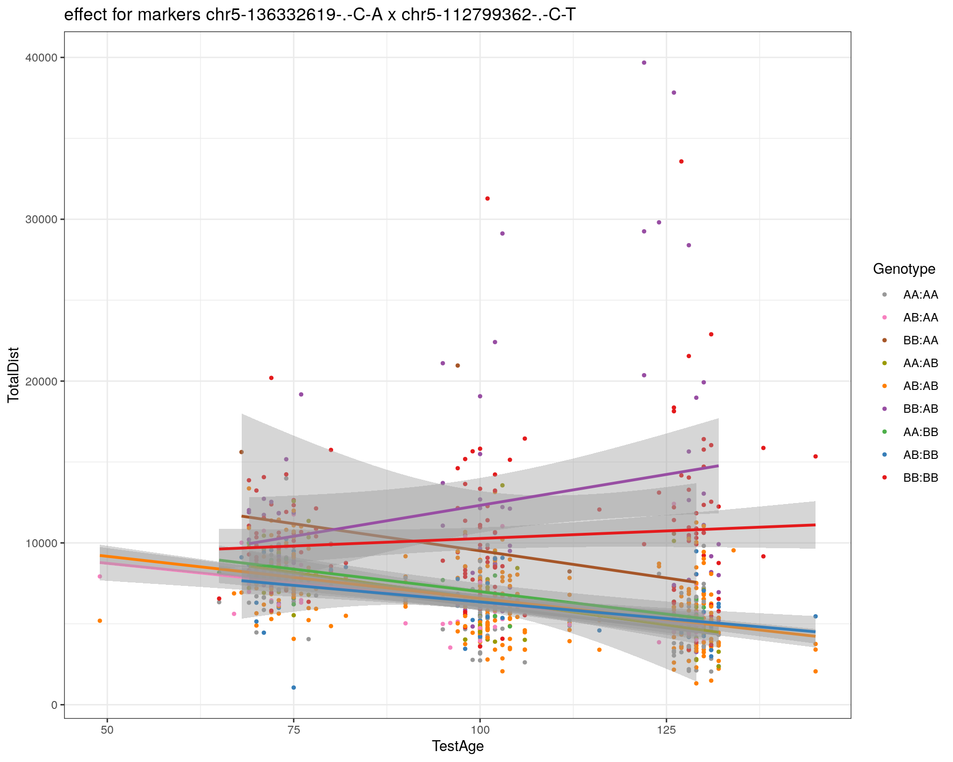

Past versions of “Plot the Dist_vs_age separate by genotype for each marker-51.png”

Version	Author	Date
2470aab	xhyuo	2022-12-24

Past versions of “Plot the Dist_vs_age separate by genotype for each marker-52.png”

Version	Author	Date
2470aab	xhyuo	2022-12-24

[1] "chr5-120660771-.-T-A"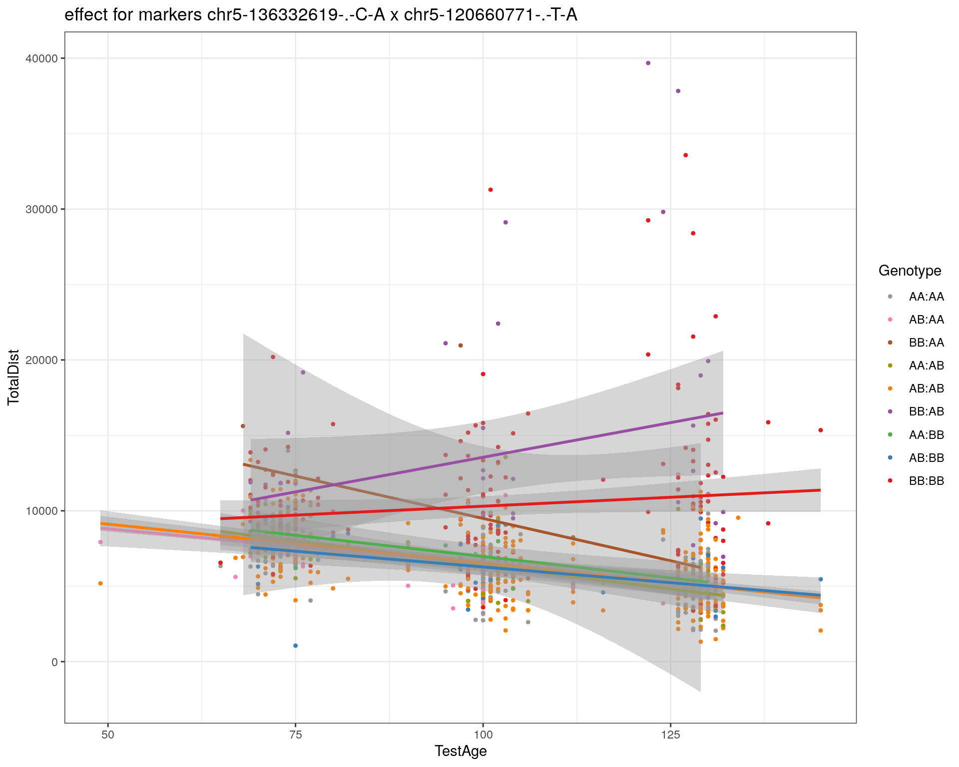

Past versions of “Plot the Dist_vs_age separate by genotype for each marker-53.png”

Version	Author	Date
2470aab	xhyuo	2022-12-24

Past versions of “Plot the Dist_vs_age separate by genotype for each marker-54.png”

Version	Author	Date
2470aab	xhyuo	2022-12-24

[1] "chr5-122167749-.-T-C"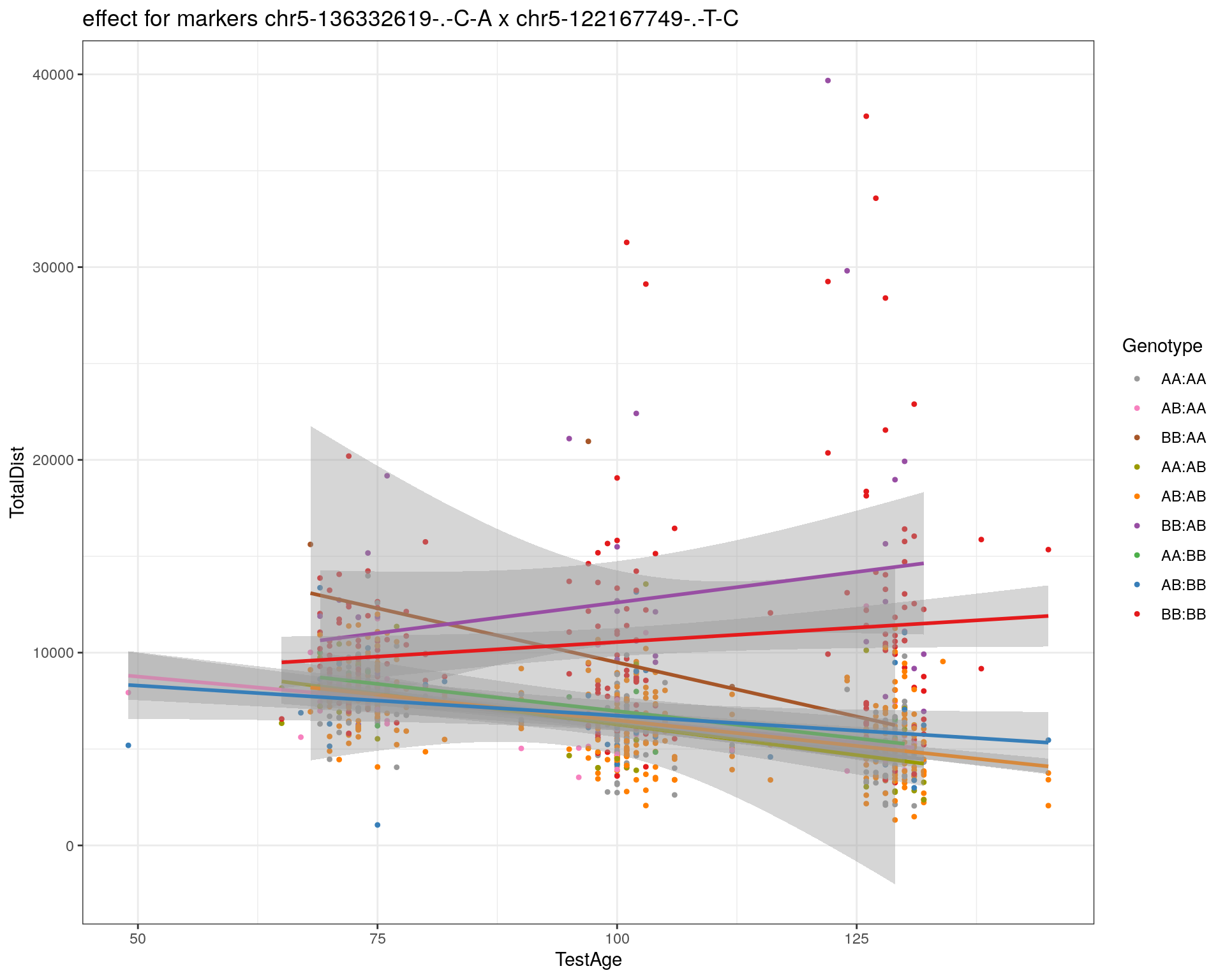

Past versions of “Plot the Dist_vs_age separate by genotype for each marker-55.png”

Version	Author	Date
2470aab	xhyuo	2022-12-24

Past versions of “Plot the Dist_vs_age separate by genotype for each marker-56.png”

Version	Author	Date
2470aab	xhyuo	2022-12-24

[1] "chr5-125153901-.-C-T"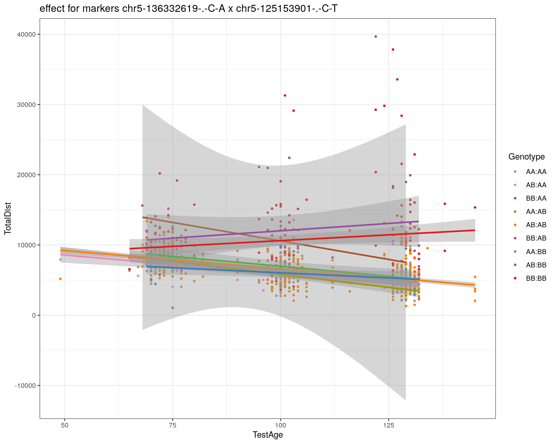

Past versions of “Plot the Dist_vs_age separate by genotype for each marker-57.png”

Version	Author	Date
2470aab	xhyuo	2022-12-24

Past versions of “Plot the Dist_vs_age separate by genotype for each marker-58.png”

Version	Author	Date
2470aab	xhyuo	2022-12-24

[1] "chr5-126058493-.-T-A"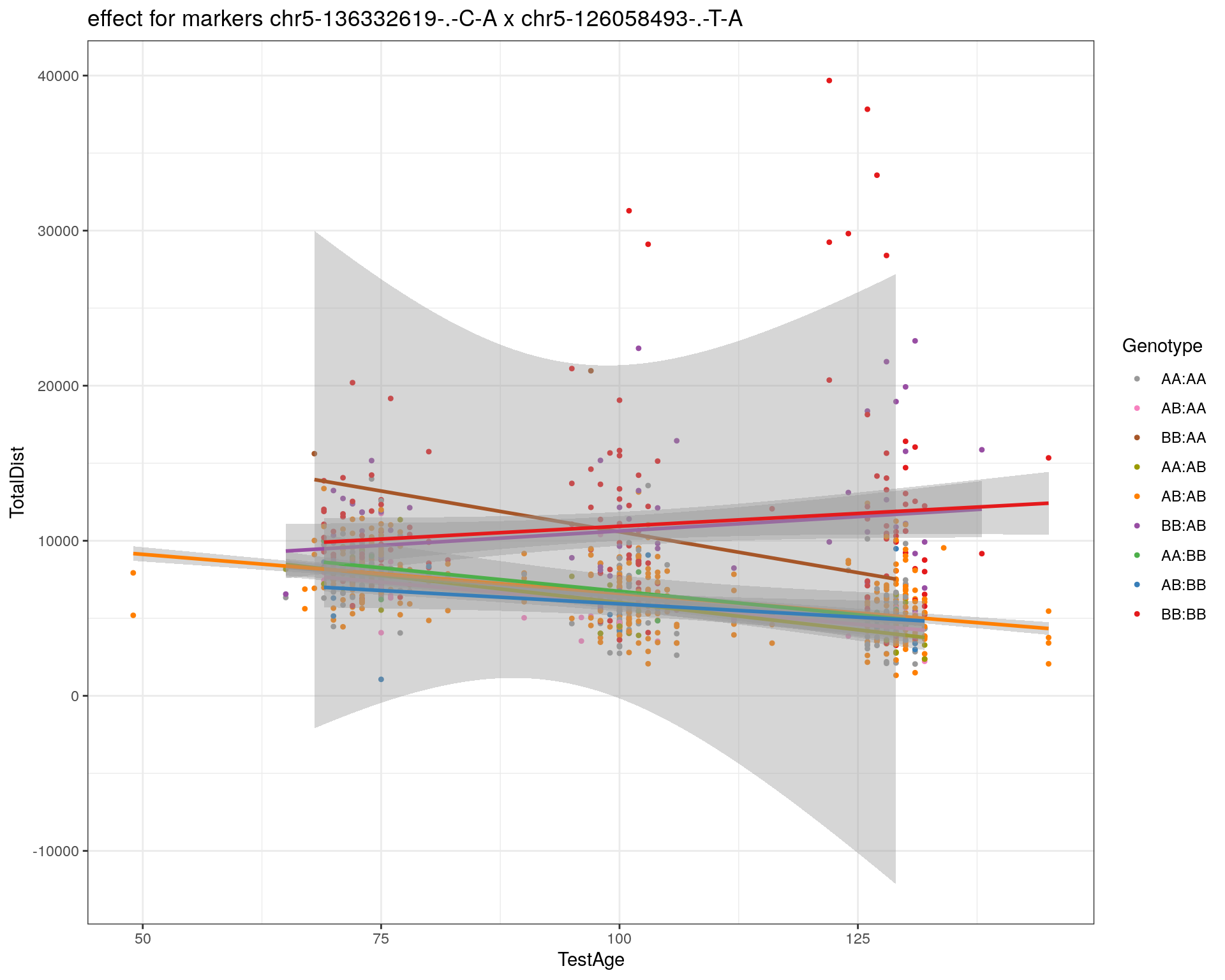

Past versions of “Plot the Dist_vs_age separate by genotype for each marker-59.png”

Version	Author	Date
2470aab	xhyuo	2022-12-24

Past versions of “Plot the Dist_vs_age separate by genotype for each marker-60.png”

Version	Author	Date
2470aab	xhyuo	2022-12-24

[1] "chr5-126551890-.-T-A"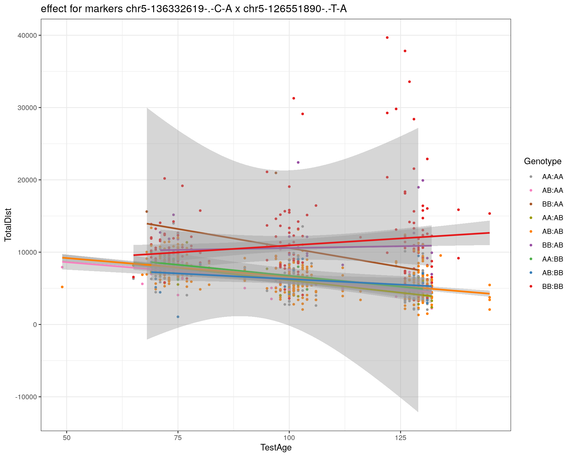

Past versions of “Plot the Dist_vs_age separate by genotype for each marker-61.png”

Version	Author	Date
2470aab	xhyuo	2022-12-24

Past versions of “Plot the Dist_vs_age separate by genotype for each marker-62.png”

Version	Author	Date
2470aab	xhyuo	2022-12-24

[1] "chr5-127565504-.-T-A"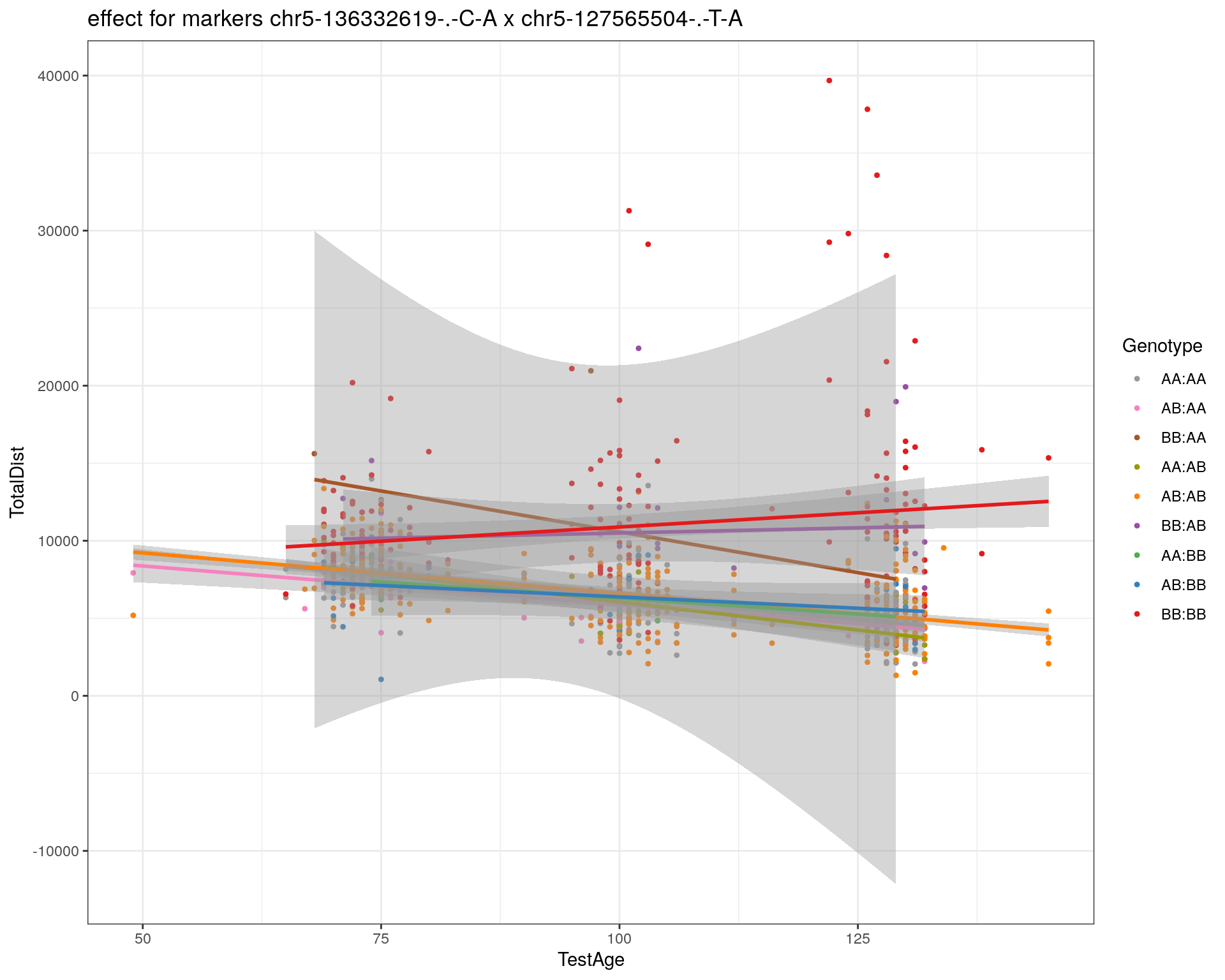

Past versions of “Plot the Dist_vs_age separate by genotype for each marker-63.png”

Version	Author	Date
2470aab	xhyuo	2022-12-24

Past versions of “Plot the Dist_vs_age separate by genotype for each marker-64.png”

Version	Author	Date
2470aab	xhyuo	2022-12-24

[1] "chr5-130394596-.-T-C"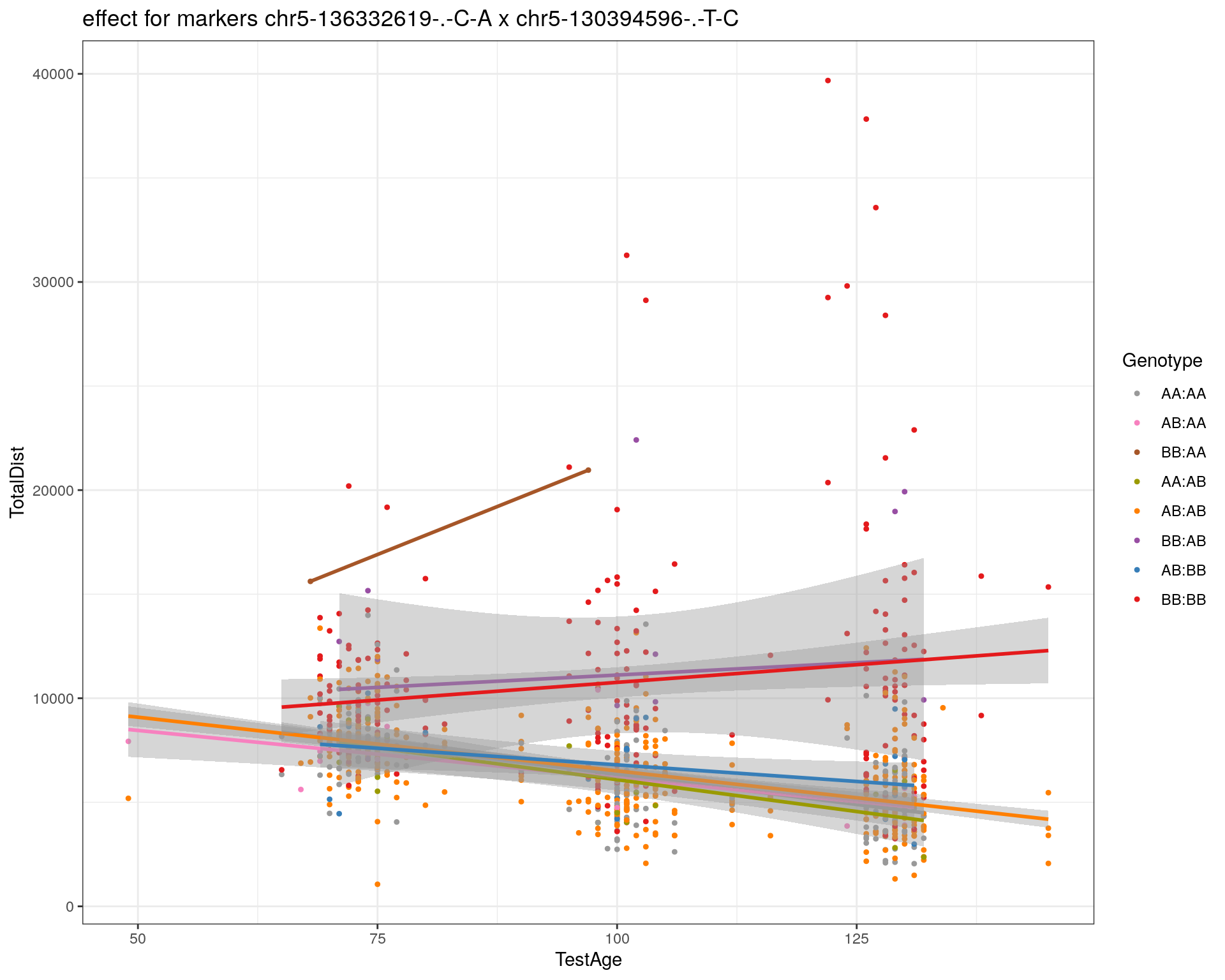

Past versions of “Plot the Dist_vs_age separate by genotype for each marker-65.png”

Version	Author	Date
2470aab	xhyuo	2022-12-24

Past versions of “Plot the Dist_vs_age separate by genotype for each marker-66.png”

Version	Author	Date
2470aab	xhyuo	2022-12-24

[1] "chr5-130943677-.-T-A"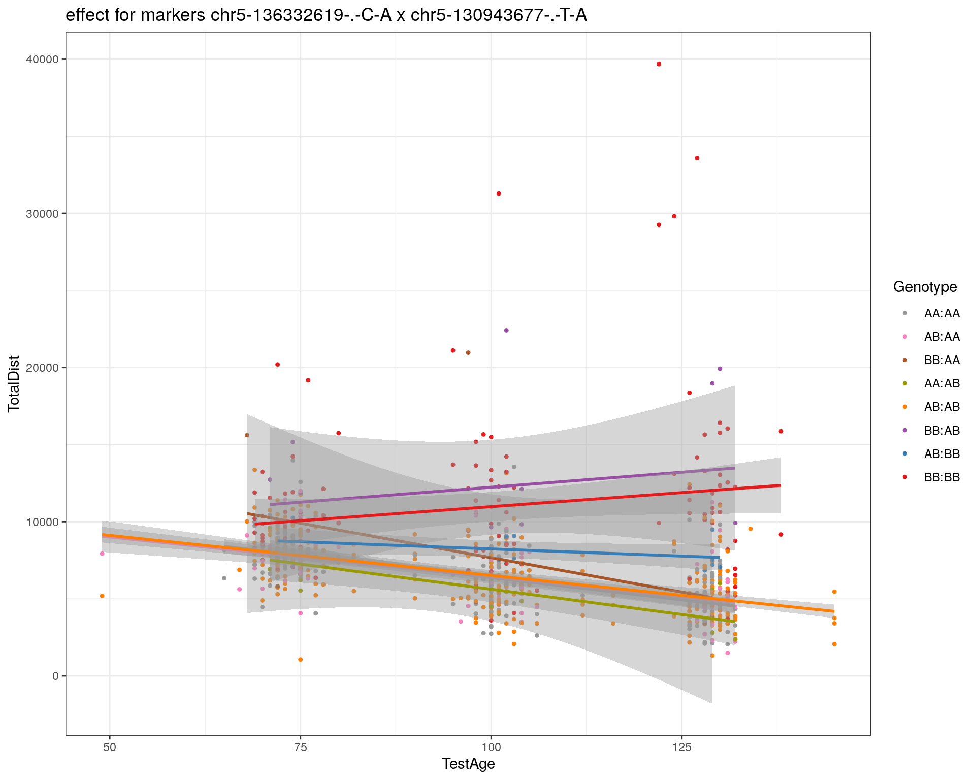

Past versions of “Plot the Dist_vs_age separate by genotype for each marker-67.png”

Version	Author	Date
2470aab	xhyuo	2022-12-24

Past versions of “Plot the Dist_vs_age separate by genotype for each marker-68.png”

Version	Author	Date
2470aab	xhyuo	2022-12-24

[1] "chr5-131298836-.-T-C"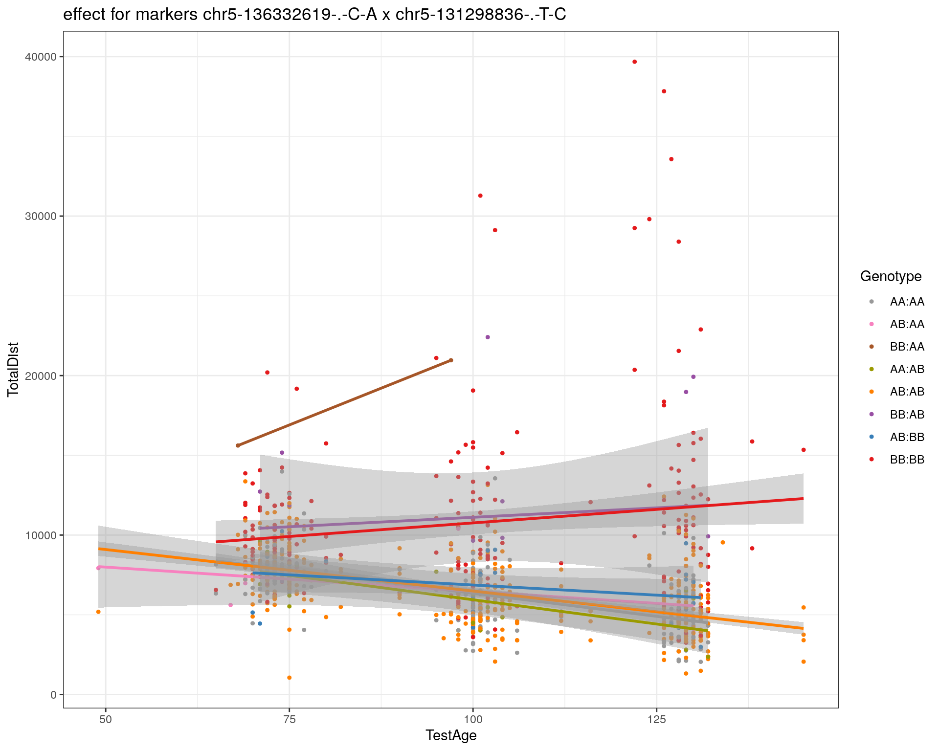

Past versions of “Plot the Dist_vs_age separate by genotype for each marker-69.png”

Version	Author	Date
2470aab	xhyuo	2022-12-24

Past versions of “Plot the Dist_vs_age separate by genotype for each marker-70.png”

Version	Author	Date
2470aab	xhyuo	2022-12-24

[1] "chr5-133052642-.-T-G"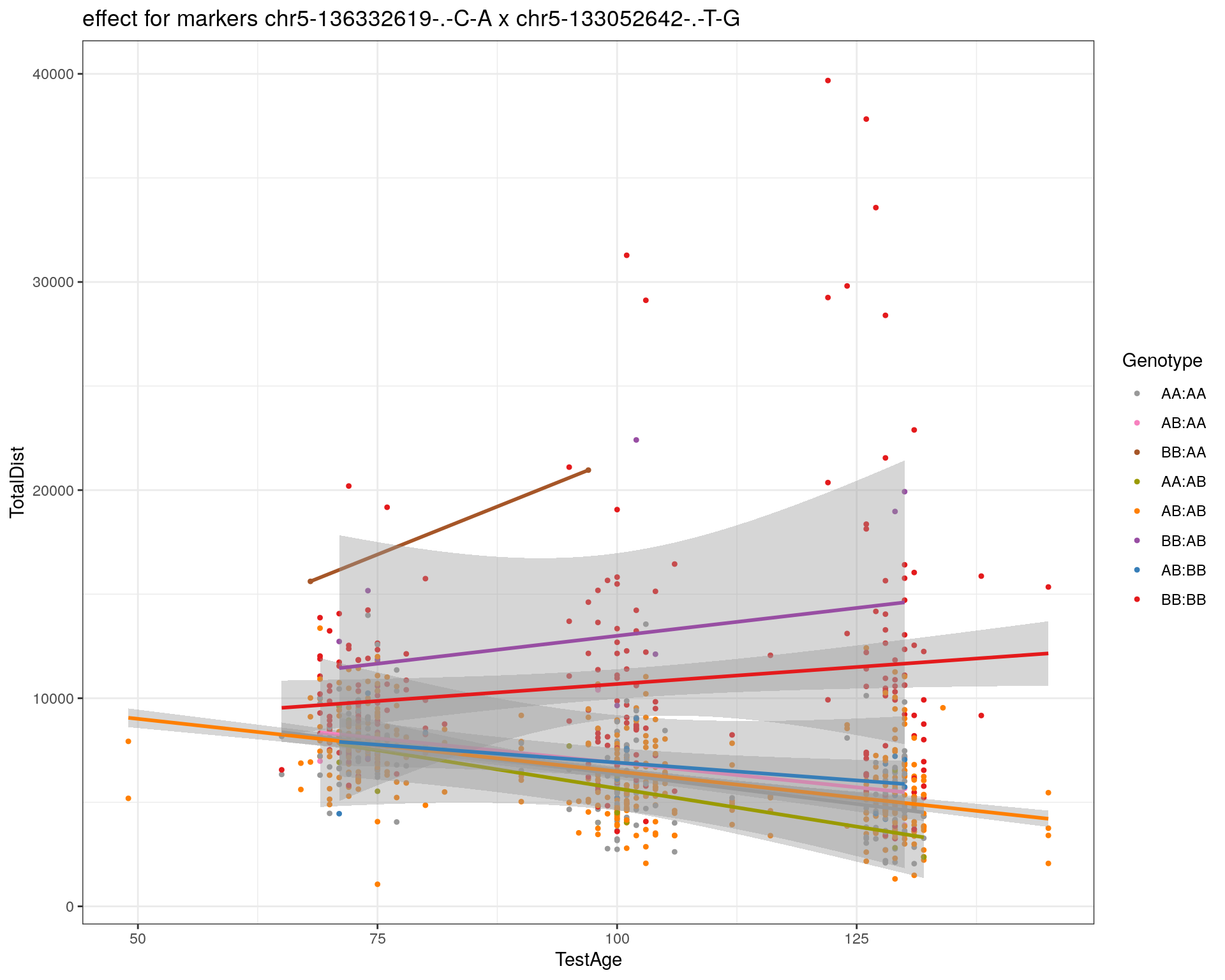

Past versions of “Plot the Dist_vs_age separate by genotype for each marker-71.png”

Version	Author	Date
2470aab	xhyuo	2022-12-24

Past versions of “Plot the Dist_vs_age separate by genotype for each marker-72.png”

Version	Author	Date
2470aab	xhyuo	2022-12-24

[1] "chr5-135960983-.-T-C"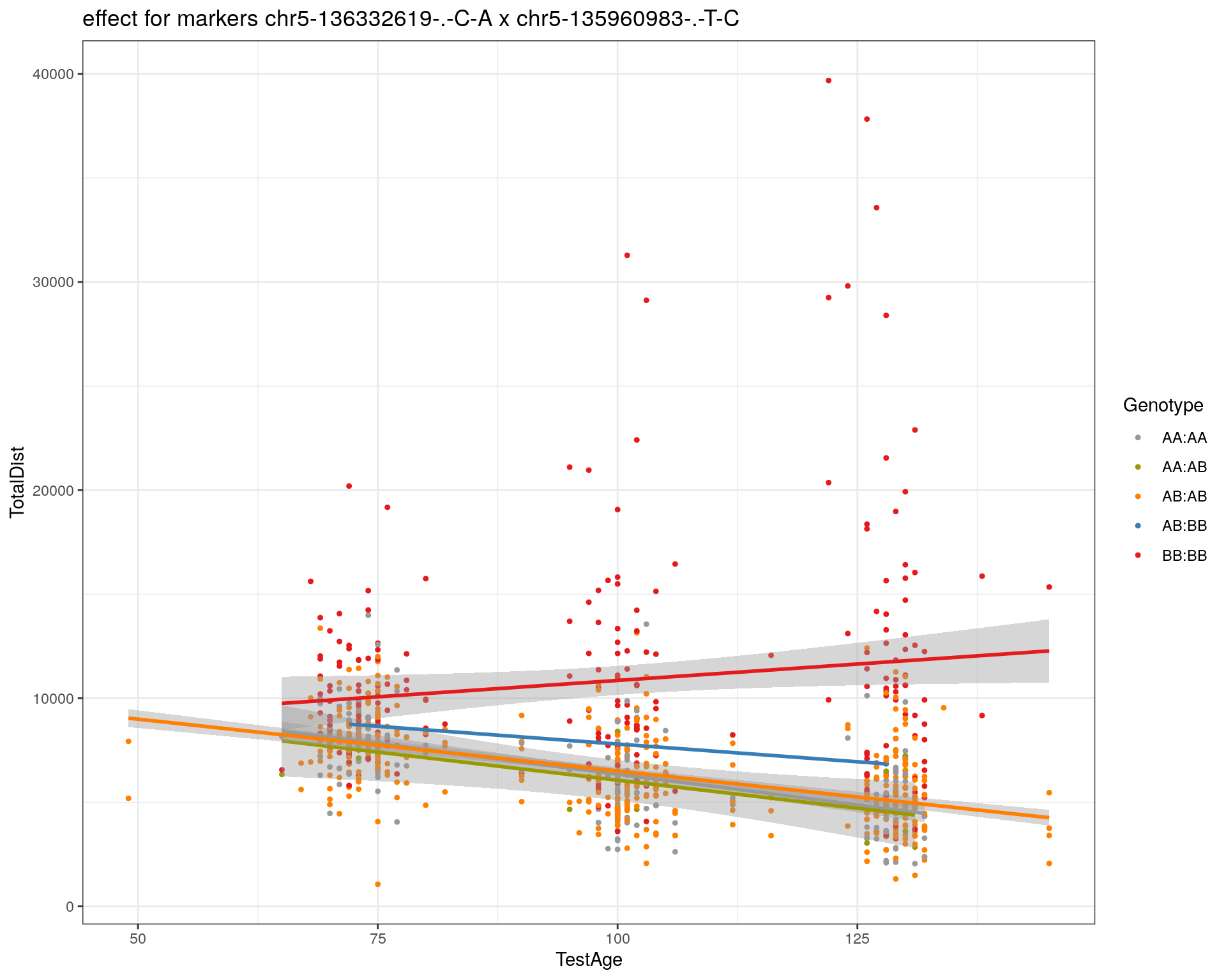

Past versions of “Plot the Dist_vs_age separate by genotype for each marker-73.png”

Version	Author	Date
2470aab	xhyuo	2022-12-24

Past versions of “Plot the Dist_vs_age separate by genotype for each marker-74.png”

Version	Author	Date
2470aab	xhyuo	2022-12-24

[1] "chr5-136332619-.-C-A"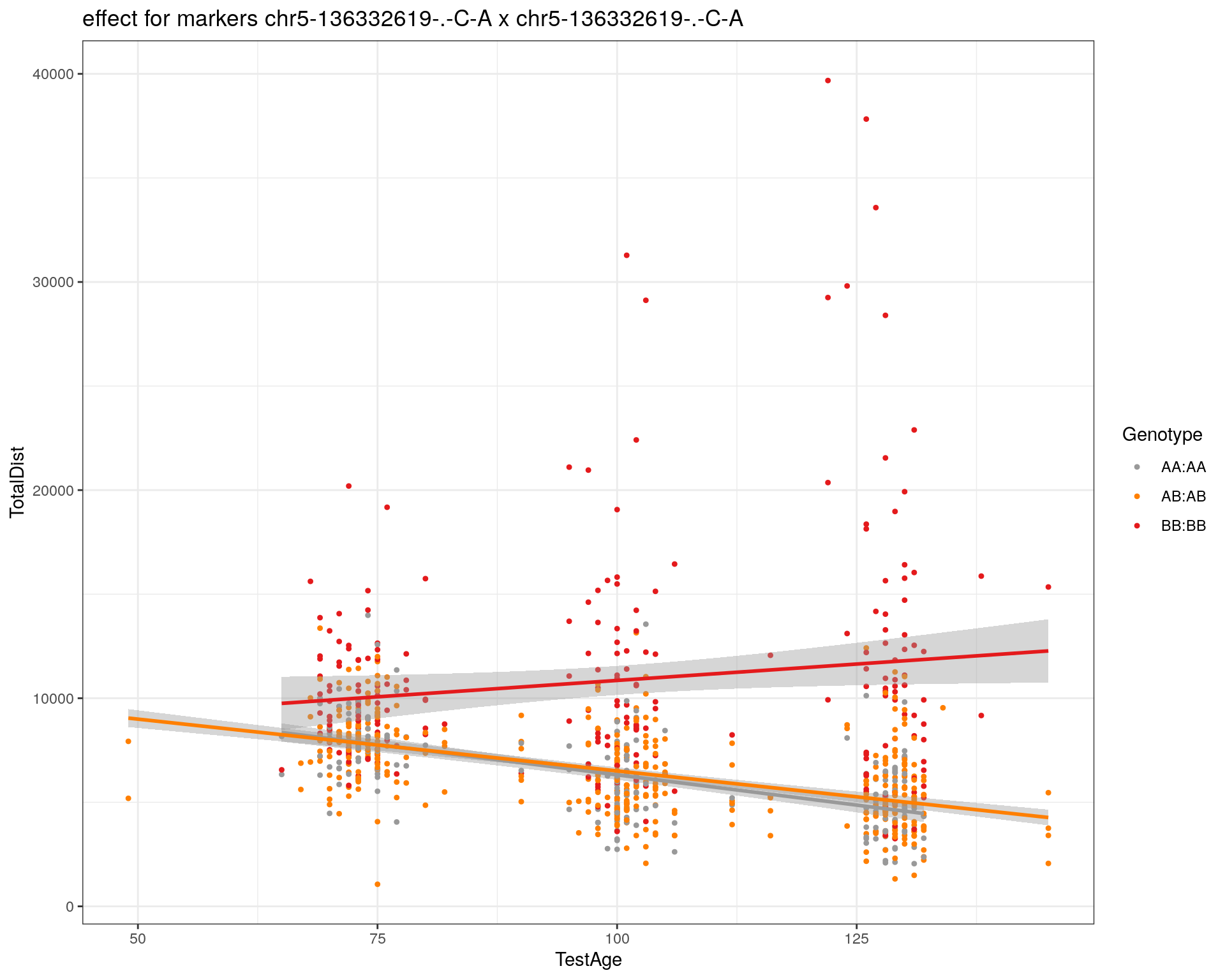

Past versions of “Plot the Dist_vs_age separate by genotype for each marker-75.png”

Version	Author	Date
2470aab	xhyuo	2022-12-24

Past versions of “Plot the Dist_vs_age separate by genotype for each marker-76.png”

Version	Author	Date
2470aab	xhyuo	2022-12-24

[1] "chr5-136844385-.-T-G"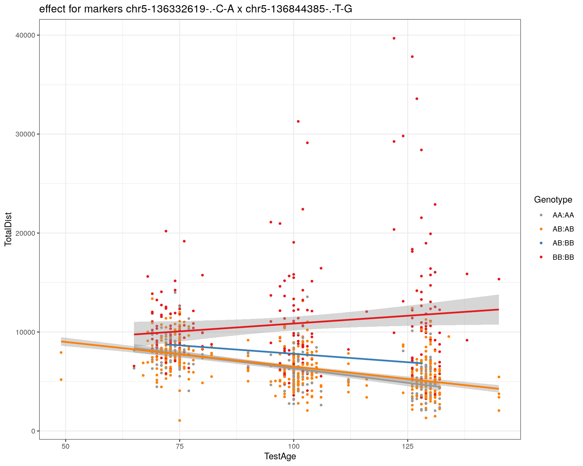

Past versions of “Plot the Dist_vs_age separate by genotype for each marker-77.png”

Version	Author	Date
2470aab	xhyuo	2022-12-24

Past versions of “Plot the Dist_vs_age separate by genotype for each marker-78.png”

Version	Author	Date
2470aab	xhyuo	2022-12-24

[1] "chr5-138956439-.-T-C"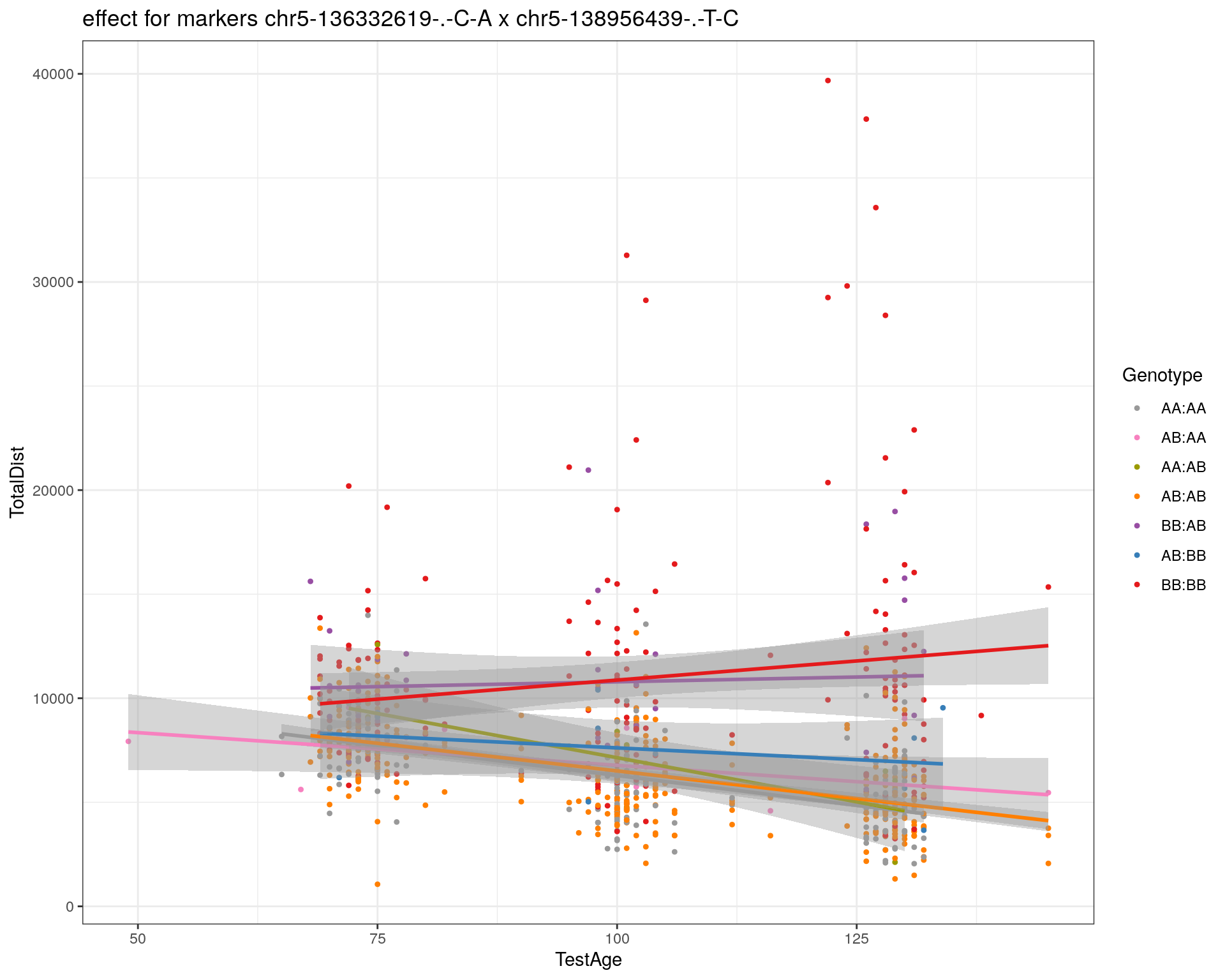

Past versions of “Plot the Dist_vs_age separate by genotype for each marker-79.png”

Version	Author	Date
2470aab	xhyuo	2022-12-24

Past versions of “Plot the Dist_vs_age separate by genotype for each marker-80.png”

Version	Author	Date
2470aab	xhyuo	2022-12-24

[1] "chr5-139706036-.-T-C"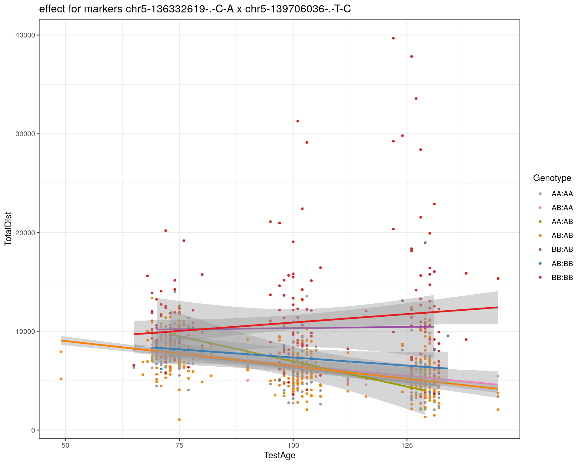

Past versions of “Plot the Dist_vs_age separate by genotype for each marker-81.png”

Version	Author	Date
2470aab	xhyuo	2022-12-24

Past versions of “Plot the Dist_vs_age separate by genotype for each marker-82.png”

Version	Author	Date
2470aab	xhyuo	2022-12-24

[1] "chr5-139891407-.-T-C"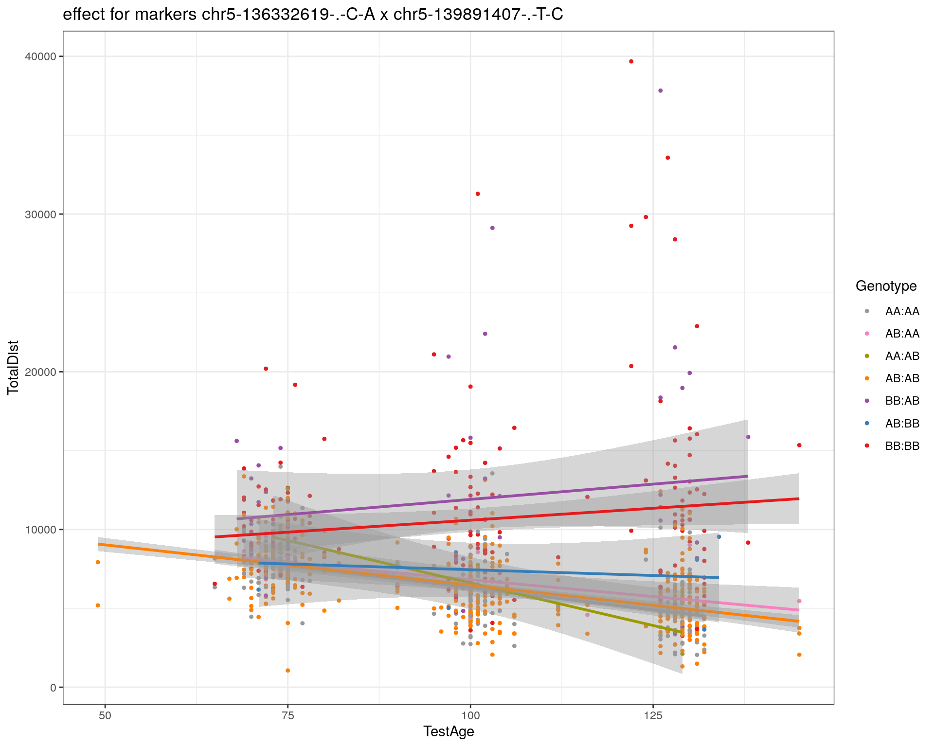

Past versions of “Plot the Dist_vs_age separate by genotype for each marker-83.png”

Version	Author	Date
2470aab	xhyuo	2022-12-24

Past versions of “Plot the Dist_vs_age separate by genotype for each marker-84.png”

Version	Author	Date
2470aab	xhyuo	2022-12-24

[1] "chr5-140071081-.-C-A"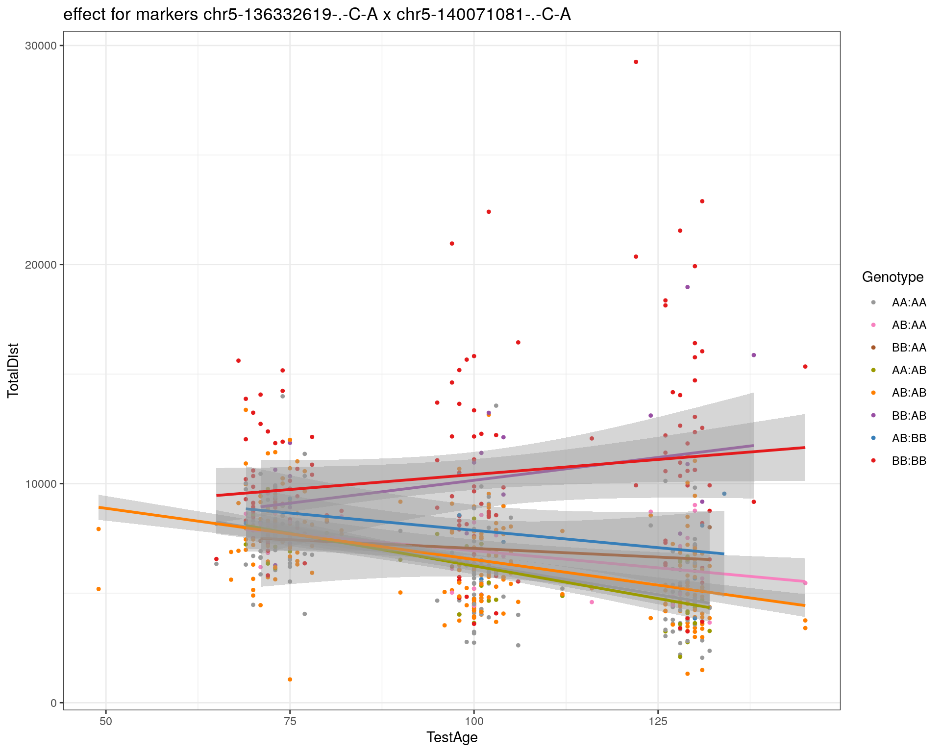

Past versions of “Plot the Dist_vs_age separate by genotype for each marker-85.png”

Version	Author	Date
2470aab	xhyuo	2022-12-24

Past versions of “Plot the Dist_vs_age separate by genotype for each marker-86.png”

Version	Author	Date
2470aab	xhyuo	2022-12-24

[1] "chr7-35061547-.-A-G"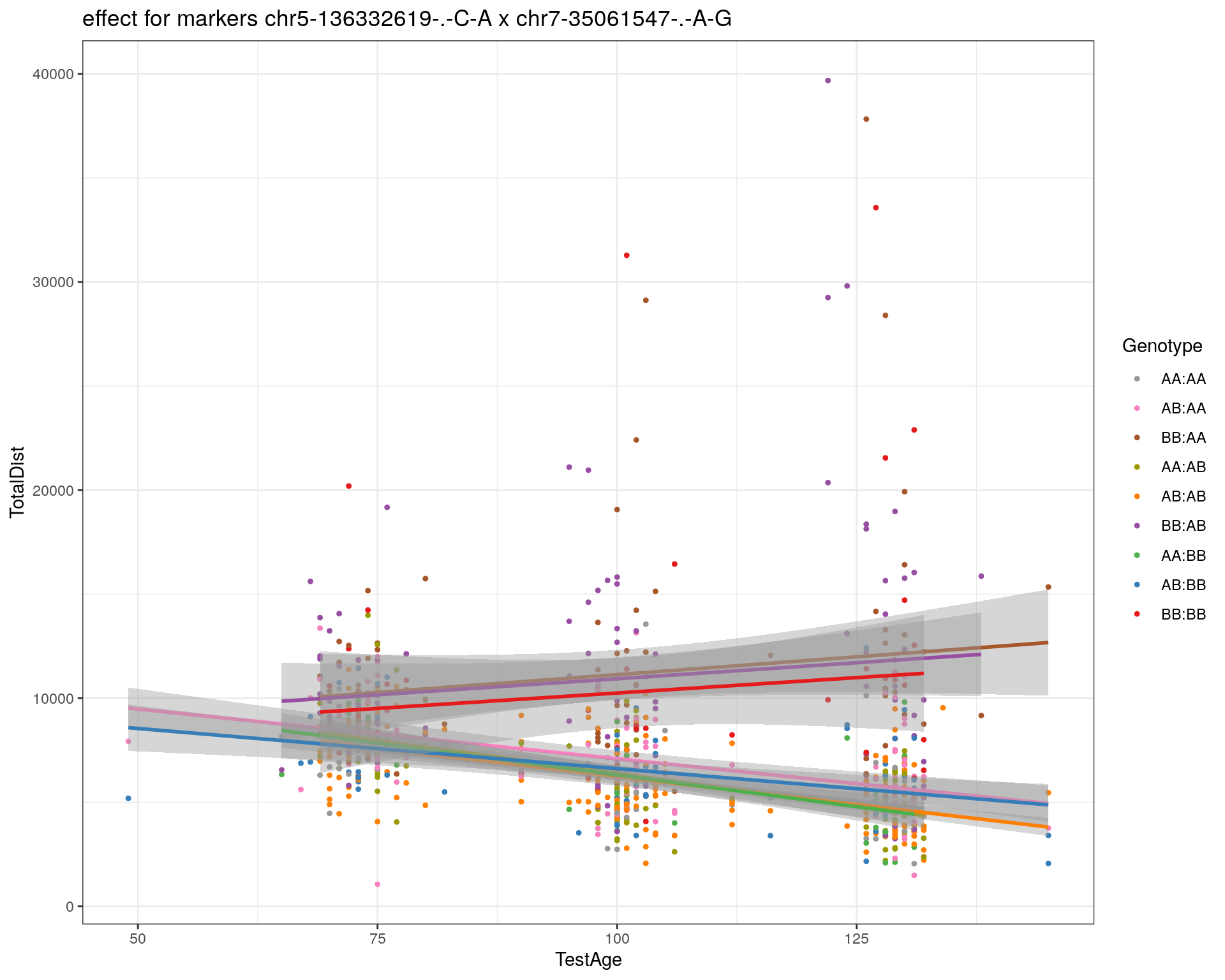

Past versions of “Plot the Dist_vs_age separate by genotype for each marker-87.png”

Version	Author	Date
2470aab	xhyuo	2022-12-24

Past versions of “Plot the Dist_vs_age separate by genotype for each marker-88.png”

Version	Author	Date
2470aab	xhyuo	2022-12-24

[1] "chr7-44272713-.-T-C"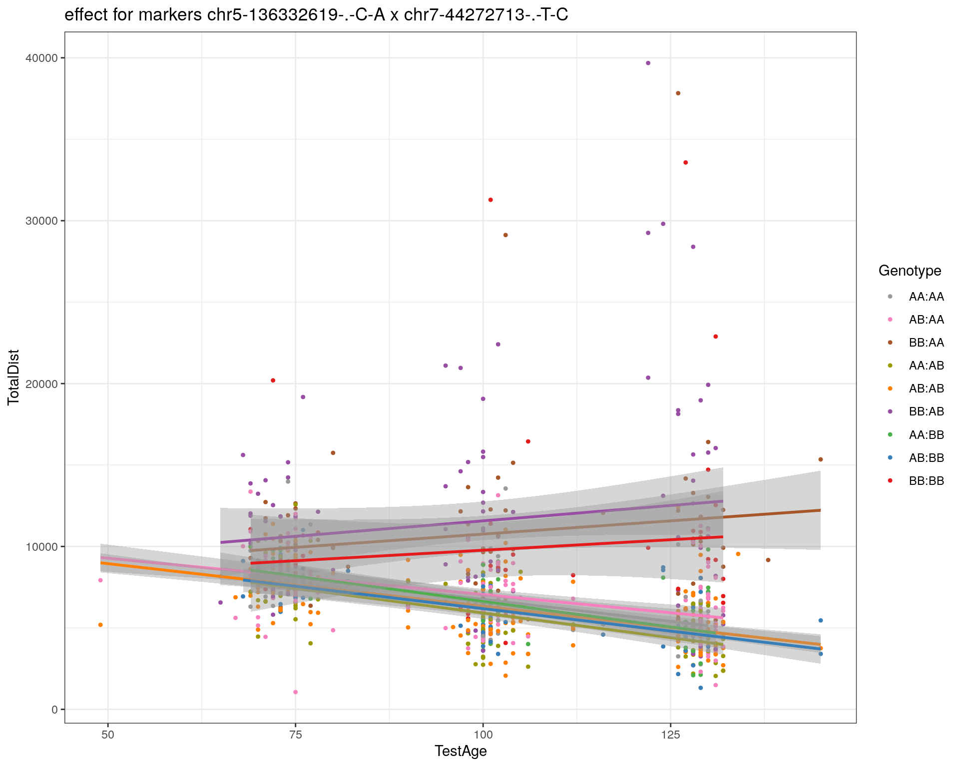

Past versions of “Plot the Dist_vs_age separate by genotype for each marker-89.png”

Version	Author	Date
2470aab	xhyuo	2022-12-24

Past versions of “Plot the Dist_vs_age separate by genotype for each marker-90.png”

Version	Author	Date
2470aab	xhyuo	2022-12-24

[1] "chr7-66785411-.-A-G"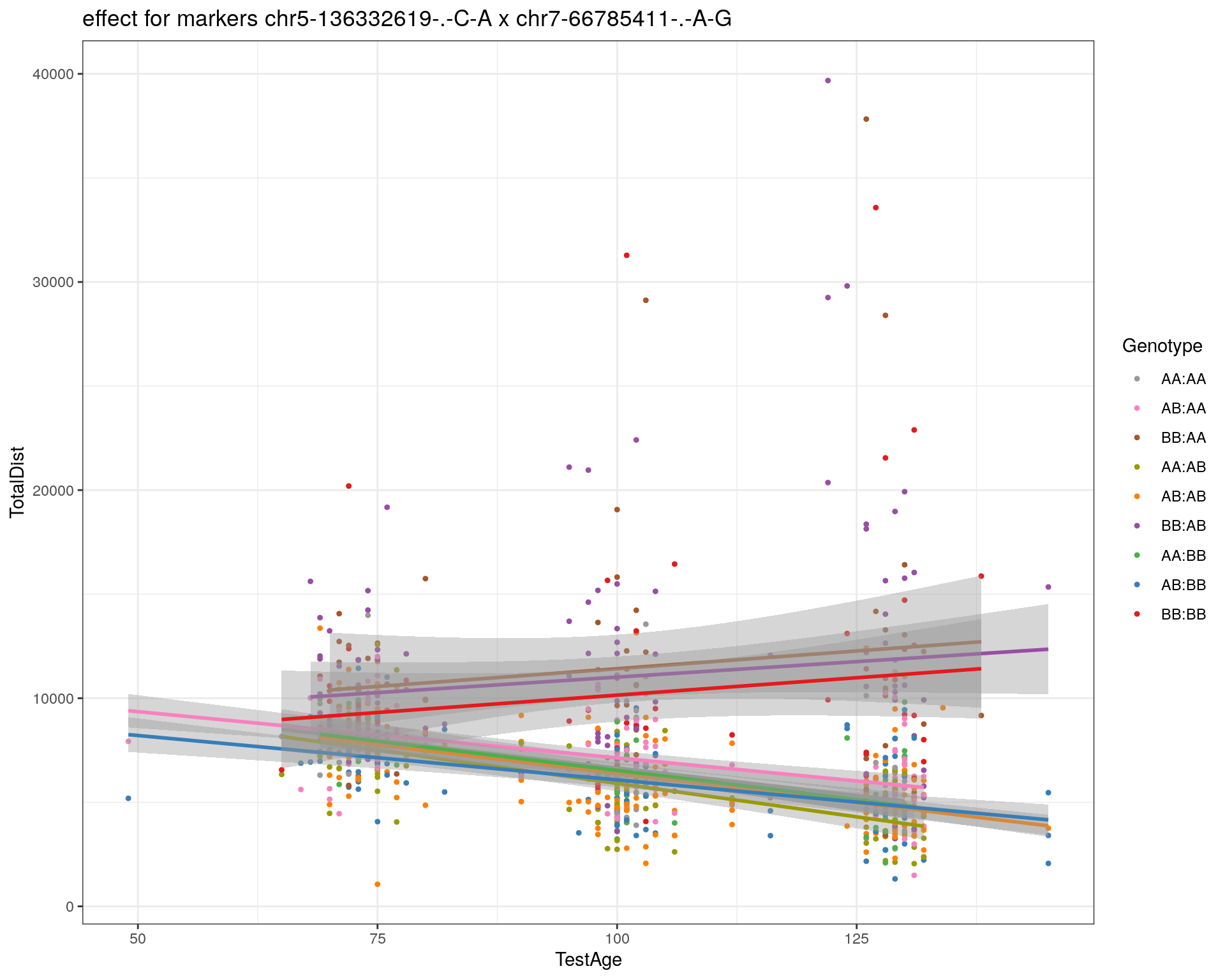

Past versions of “Plot the Dist_vs_age separate by genotype for each marker-91.png”

Version	Author	Date
2470aab	xhyuo	2022-12-24

Past versions of “Plot the Dist_vs_age separate by genotype for each marker-92.png”

Version	Author	Date
2470aab	xhyuo	2022-12-24

[1] "chr7-112510032-.-A-T"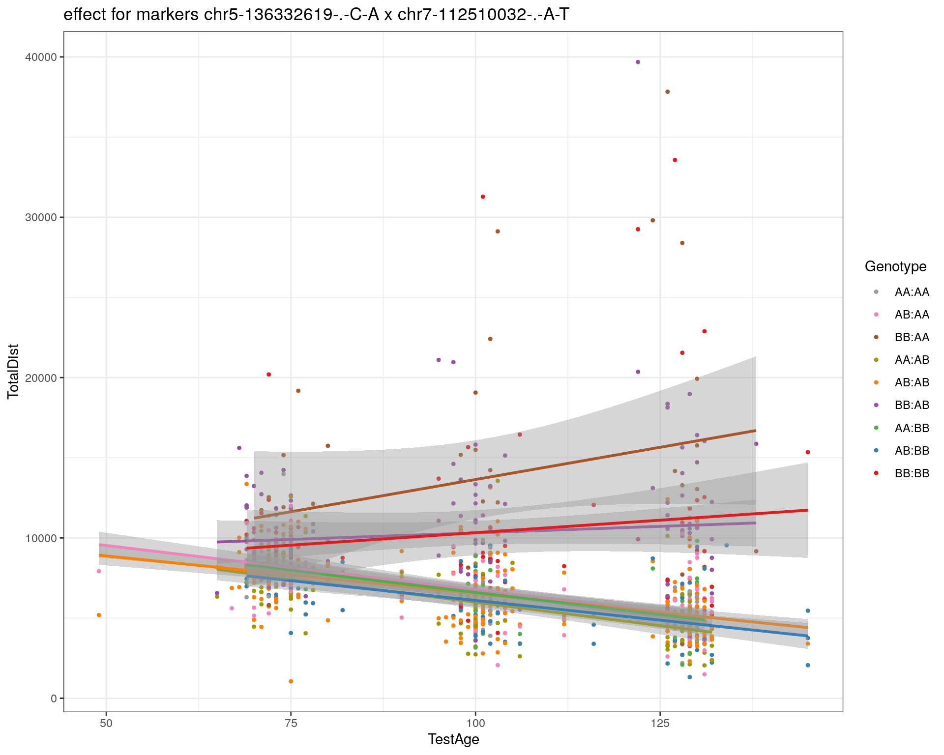

Past versions of “Plot the Dist_vs_age separate by genotype for each marker-93.png”

Version	Author	Date
2470aab	xhyuo	2022-12-24

Past versions of “Plot the Dist_vs_age separate by genotype for each marker-94.png”

Version	Author	Date
2470aab	xhyuo	2022-12-24

[1] "chr8-91986173-.-T-C"

Past versions of “Plot the Dist_vs_age separate by genotype for each marker-95.png”

Version	Author	Date
2470aab	xhyuo	2022-12-24

Past versions of “Plot the Dist_vs_age separate by genotype for each marker-96.png”

Version	Author	Date
2470aab	xhyuo	2022-12-24

[1] "chr8-99395759-.-T-C"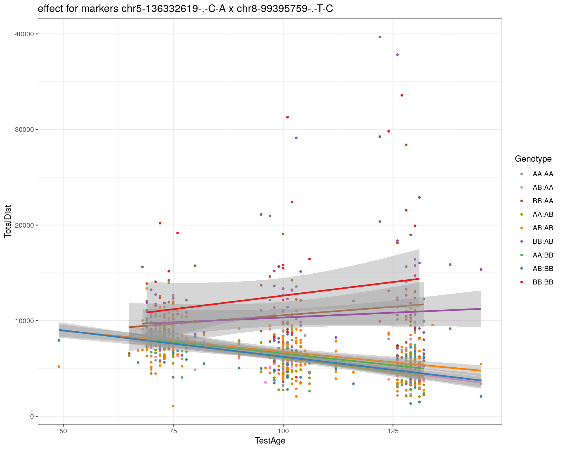

Past versions of “Plot the Dist_vs_age separate by genotype for each marker-97.png”

Version	Author	Date
2470aab	xhyuo	2022-12-24

Past versions of “Plot the Dist_vs_age separate by genotype for each marker-98.png”

Version	Author	Date
2470aab	xhyuo	2022-12-24

[1] "chr8-112465004-.-G-A"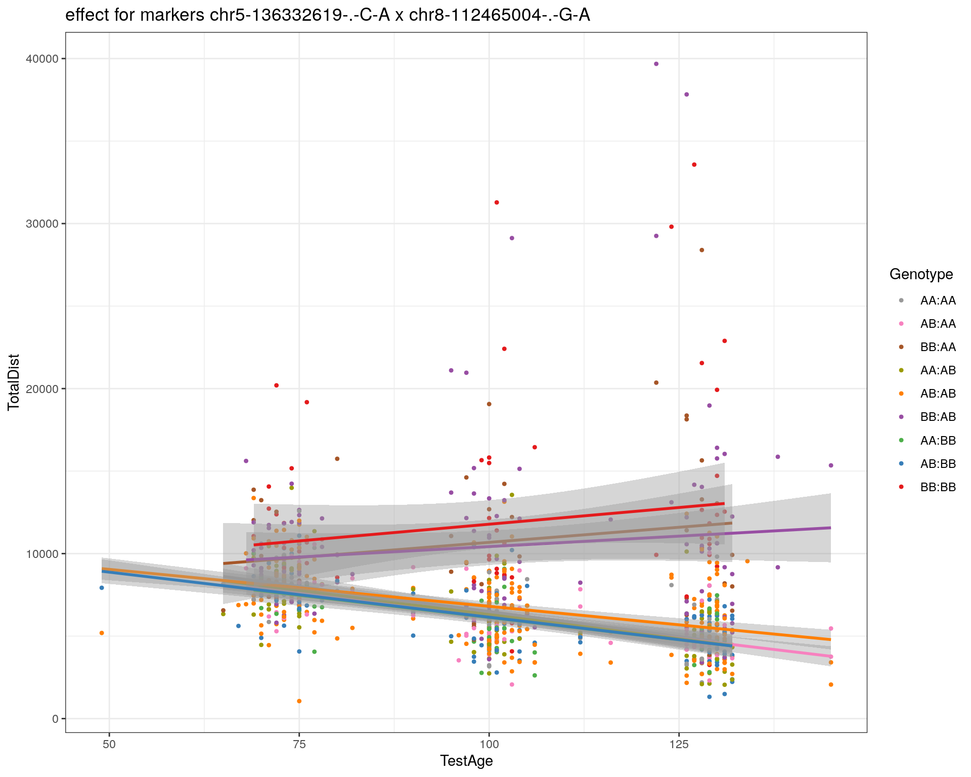

Past versions of “Plot the Dist_vs_age separate by genotype for each marker-99.png”

Version	Author	Date
2470aab	xhyuo	2022-12-24

Past versions of “Plot the Dist_vs_age separate by genotype for each marker-100.png”

Version	Author	Date
2470aab	xhyuo	2022-12-24

[1] "chr9-64698947-.-C-T"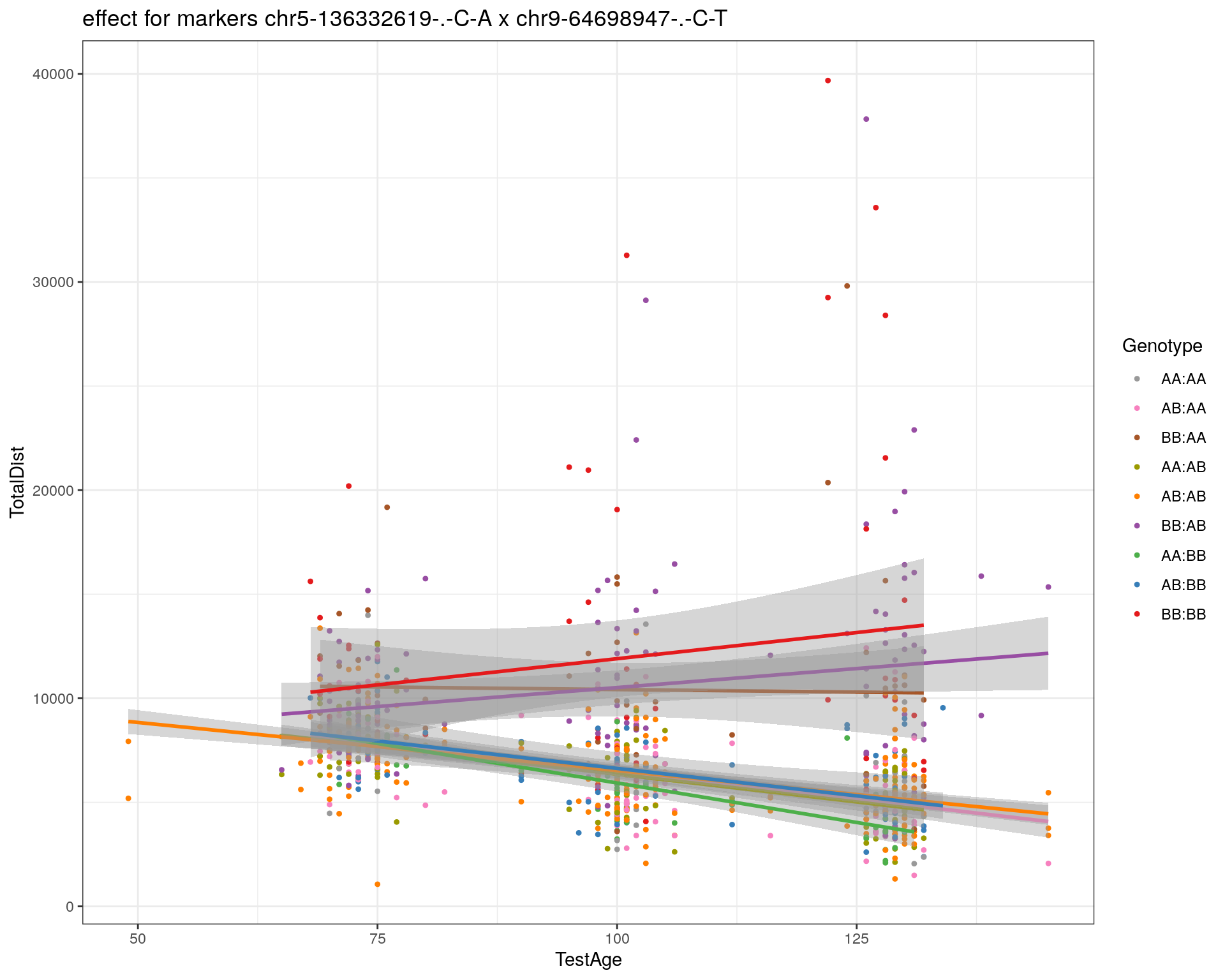

Past versions of “Plot the Dist_vs_age separate by genotype for each marker-101.png”

Version	Author	Date
2470aab	xhyuo	2022-12-24

Past versions of “Plot the Dist_vs_age separate by genotype for each marker-102.png”

Version	Author	Date
2470aab	xhyuo	2022-12-24

[1] "chr9-65857475-.-T-C"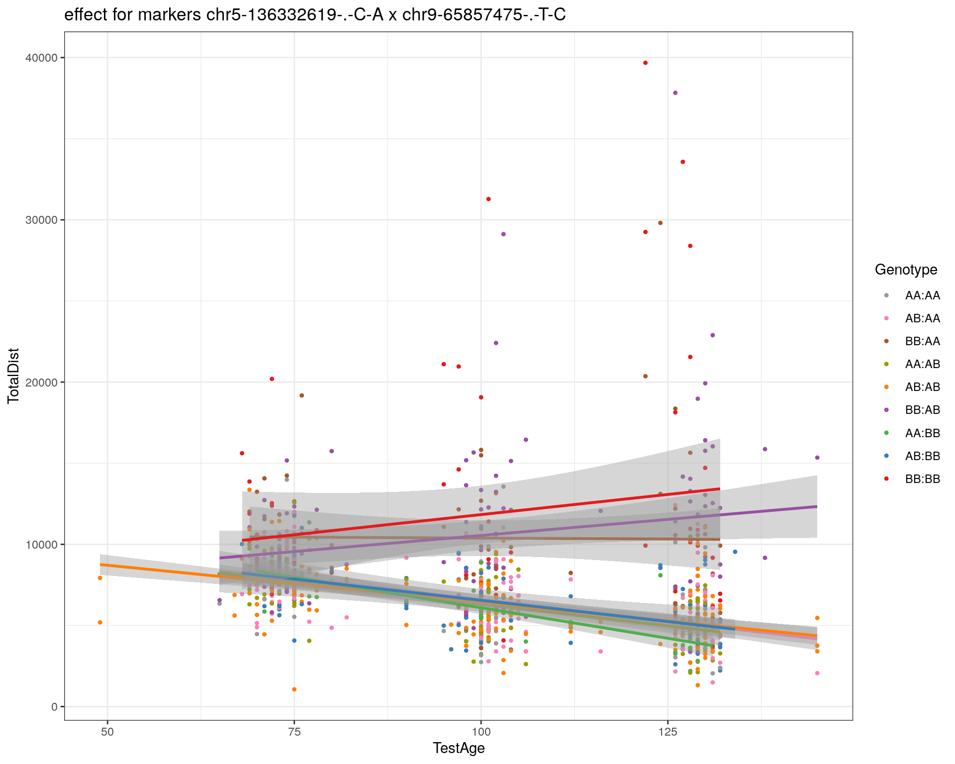

Past versions of “Plot the Dist_vs_age separate by genotype for each marker-103.png”

Version	Author	Date
2470aab	xhyuo	2022-12-24

Past versions of “Plot the Dist_vs_age separate by genotype for each marker-104.png”

Version	Author	Date
2470aab	xhyuo	2022-12-24

[1] "chr9-69415567-.-T-A"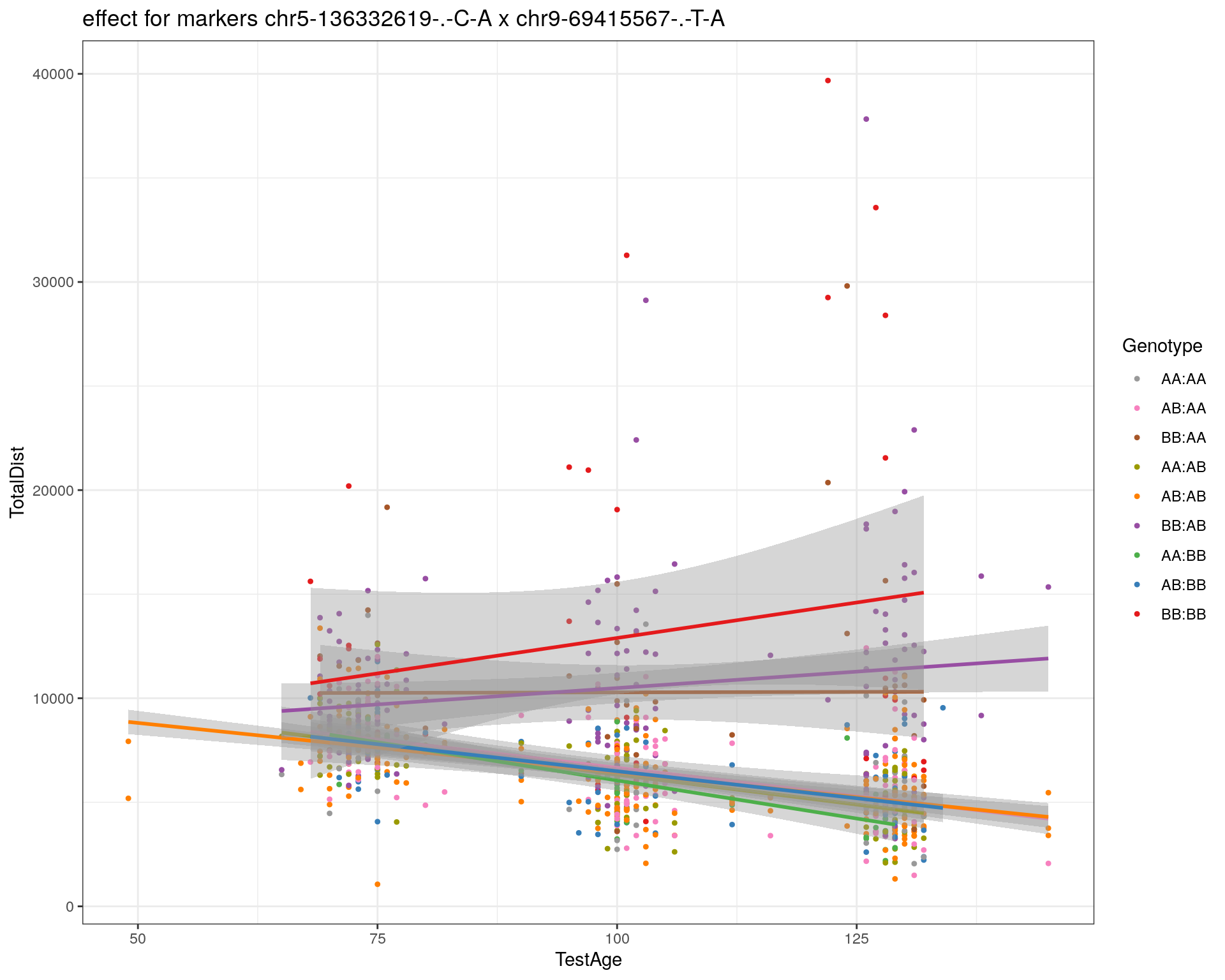

Past versions of “Plot the Dist_vs_age separate by genotype for each marker-105.png”

Version	Author	Date
2470aab	xhyuo	2022-12-24

Past versions of “Plot the Dist_vs_age separate by genotype for each marker-106.png”

Version	Author	Date
2470aab	xhyuo	2022-12-24

[1] "chr9-71739608-.-T-A"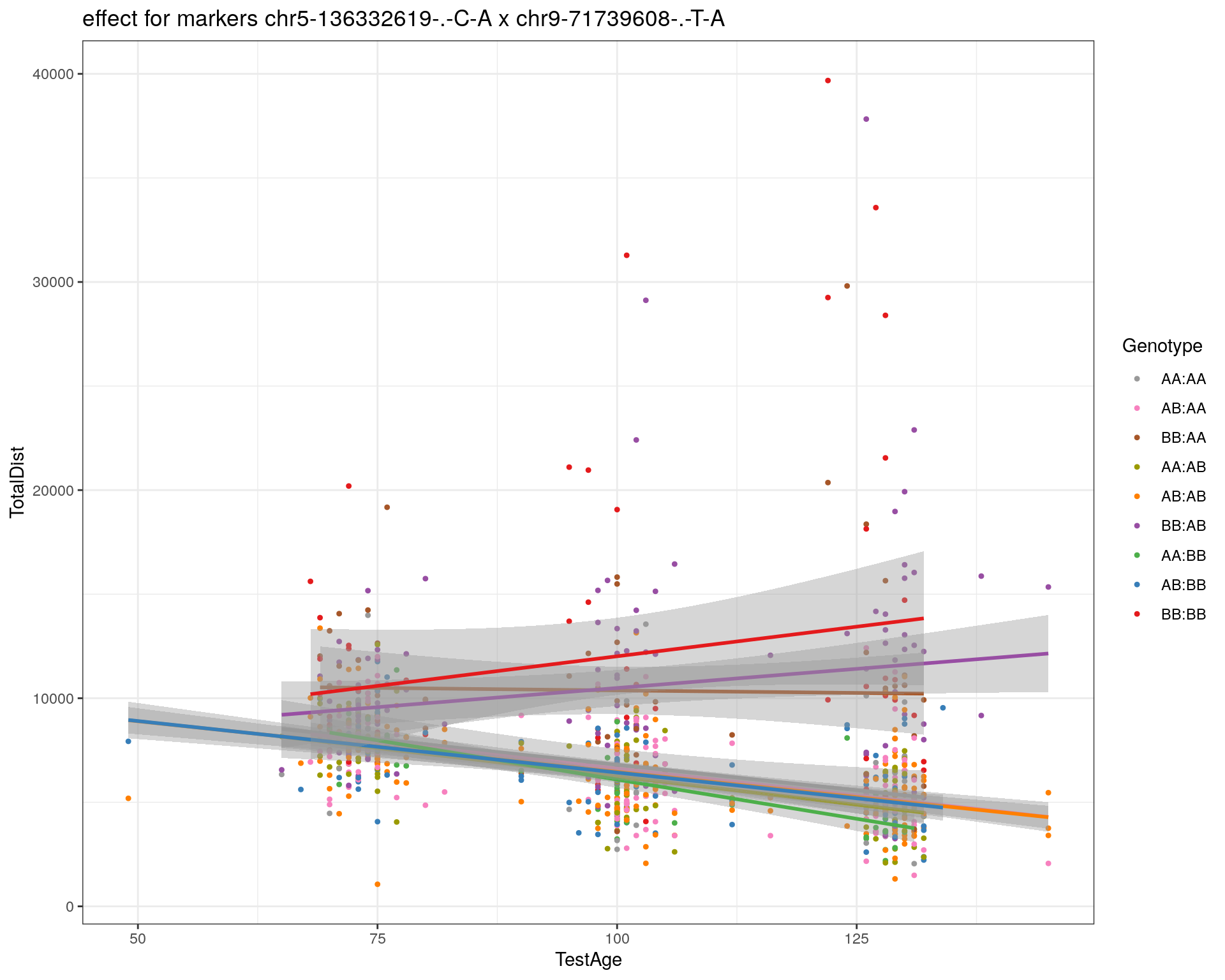

Past versions of “Plot the Dist_vs_age separate by genotype for each marker-107.png”

Version	Author	Date
2470aab	xhyuo	2022-12-24

Past versions of “Plot the Dist_vs_age separate by genotype for each marker-108.png”

Version	Author	Date
2470aab	xhyuo	2022-12-24

[1] "chr9-80465702-.-T-A"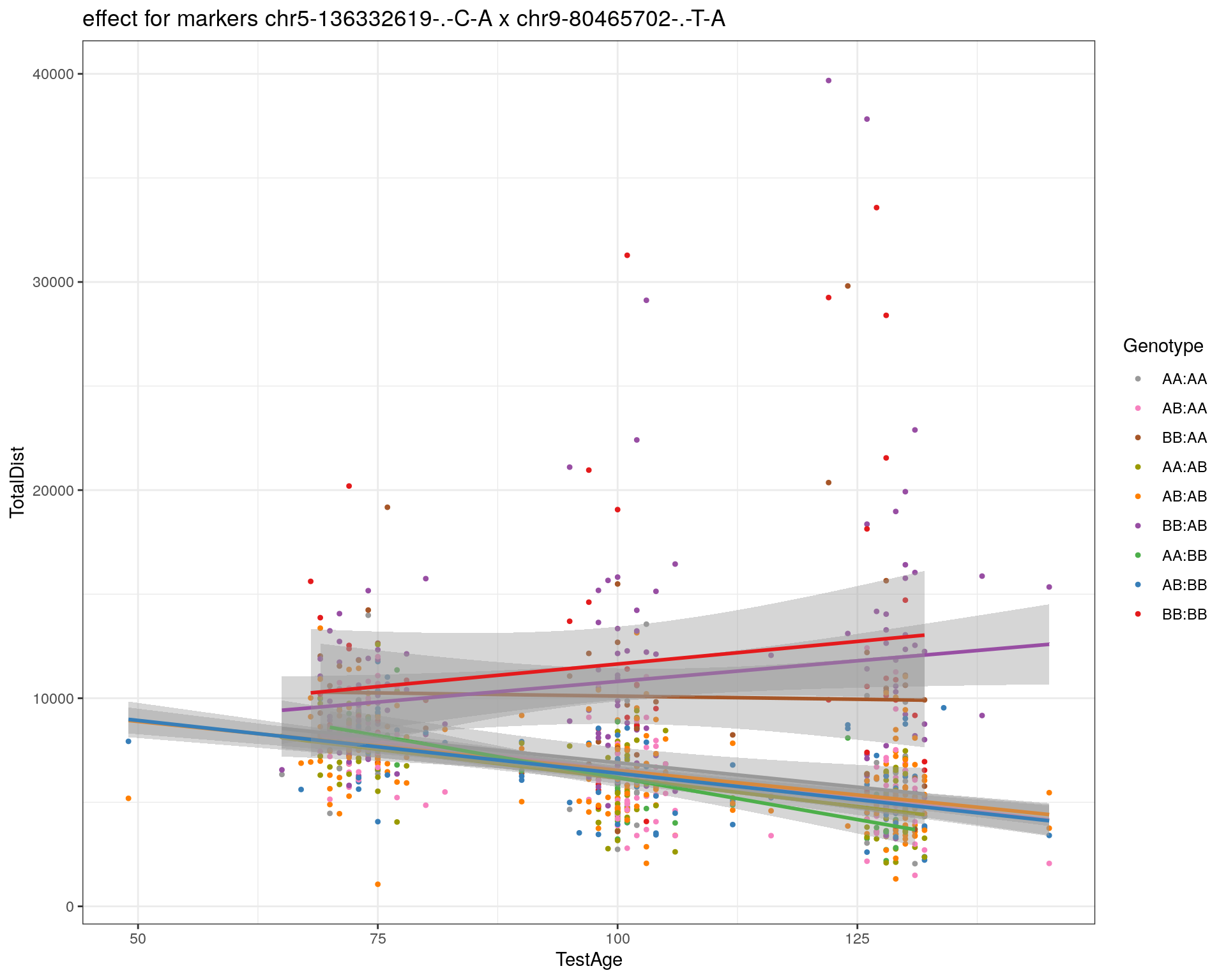

Past versions of “Plot the Dist_vs_age separate by genotype for each marker-109.png”

Version	Author	Date
2470aab	xhyuo	2022-12-24

Past versions of “Plot the Dist_vs_age separate by genotype for each marker-110.png”

Version	Author	Date
2470aab	xhyuo	2022-12-24

[1] "chr10-24134777-.-A-T"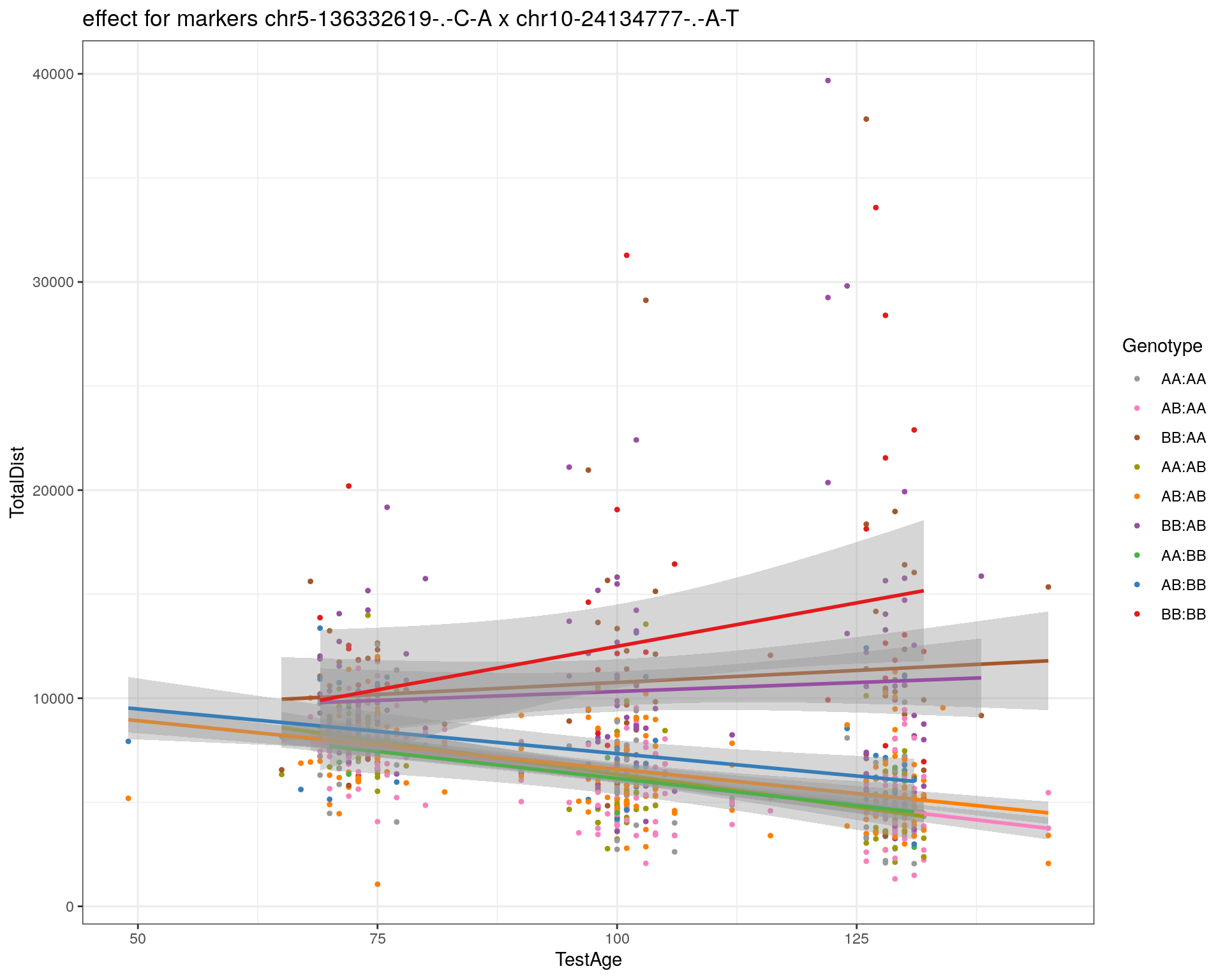

Past versions of “Plot the Dist_vs_age separate by genotype for each marker-111.png”

Version	Author	Date
2470aab	xhyuo	2022-12-24

Past versions of “Plot the Dist_vs_age separate by genotype for each marker-112.png”

Version	Author	Date
2470aab	xhyuo	2022-12-24

[1] "chr11-96730656-.-A-G"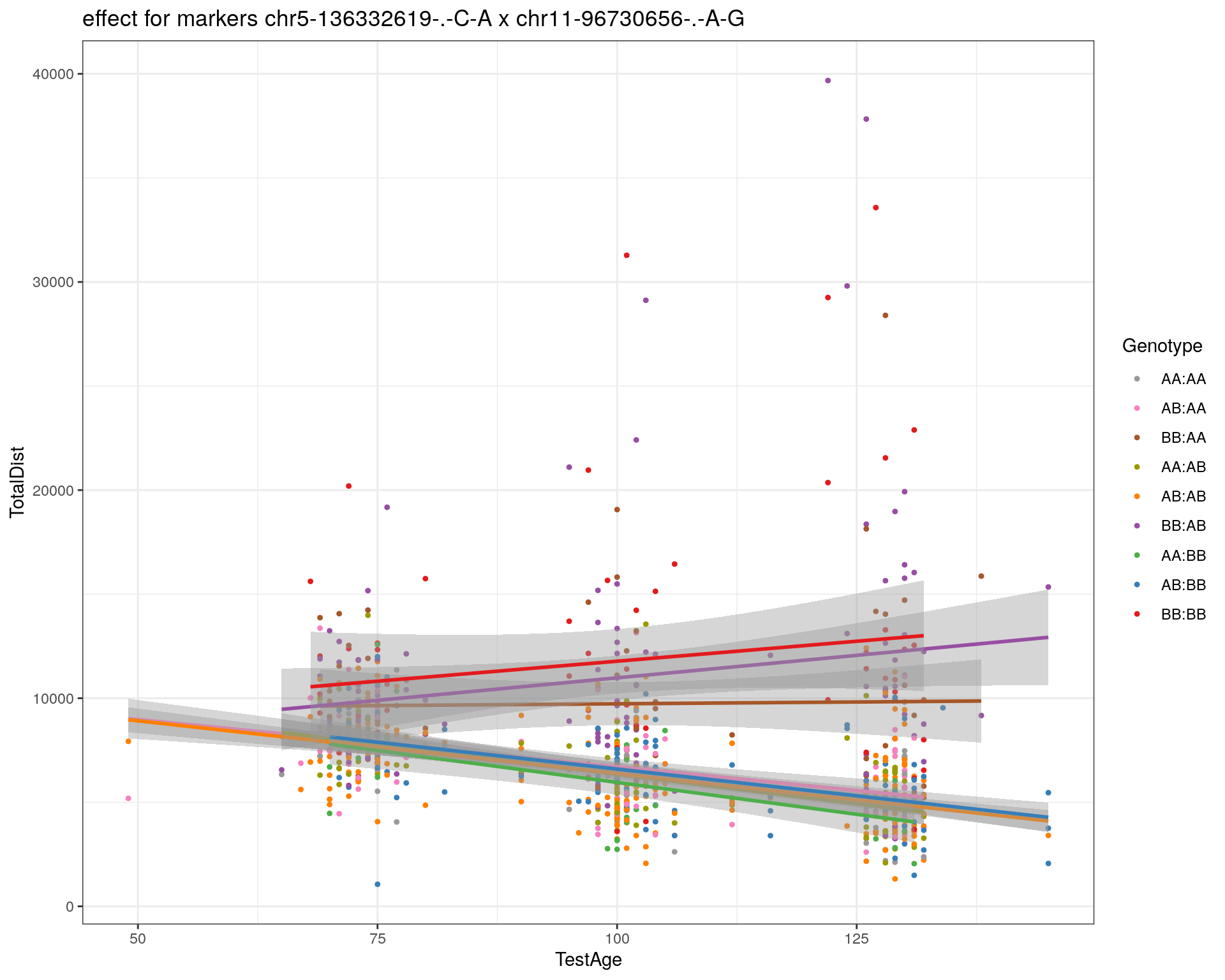

Past versions of “Plot the Dist_vs_age separate by genotype for each marker-113.png”

Version	Author	Date
2470aab	xhyuo	2022-12-24

Past versions of “Plot the Dist_vs_age separate by genotype for each marker-114.png”

Version	Author	Date
2470aab	xhyuo	2022-12-24

[1] "chr12-43136399-.-A-T"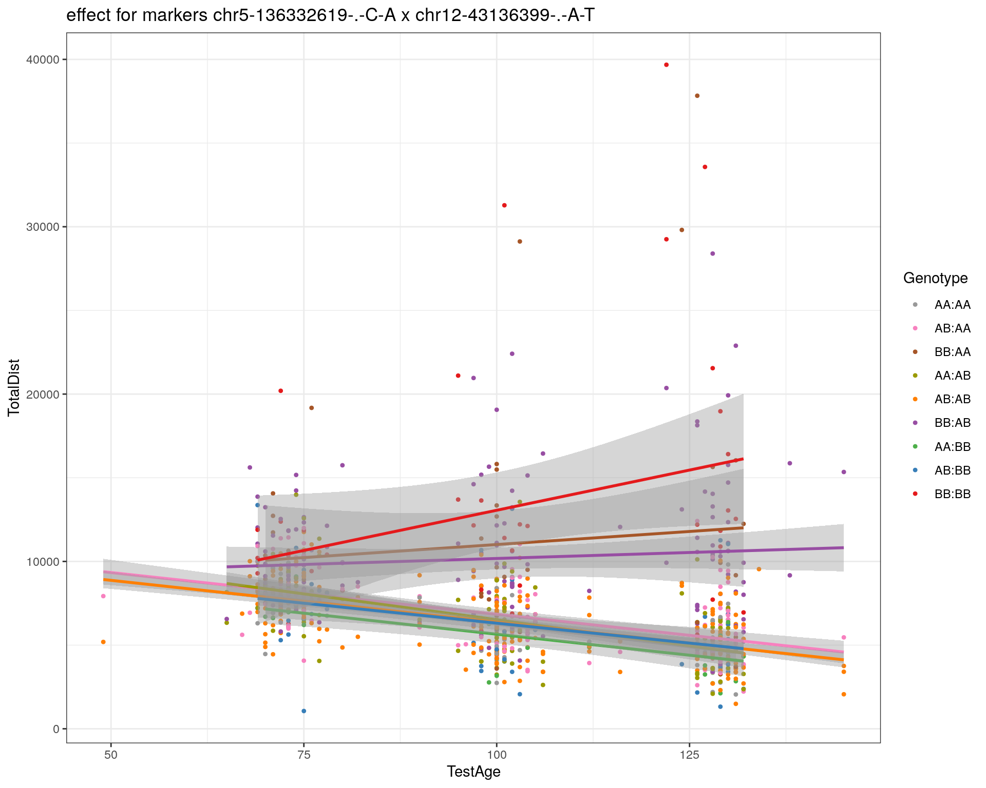

Past versions of “Plot the Dist_vs_age separate by genotype for each marker-115.png”

Version	Author	Date
2470aab	xhyuo	2022-12-24

Past versions of “Plot the Dist_vs_age separate by genotype for each marker-116.png”

Version	Author	Date
2470aab	xhyuo	2022-12-24

[1] "chr12-69197484-.-C-A"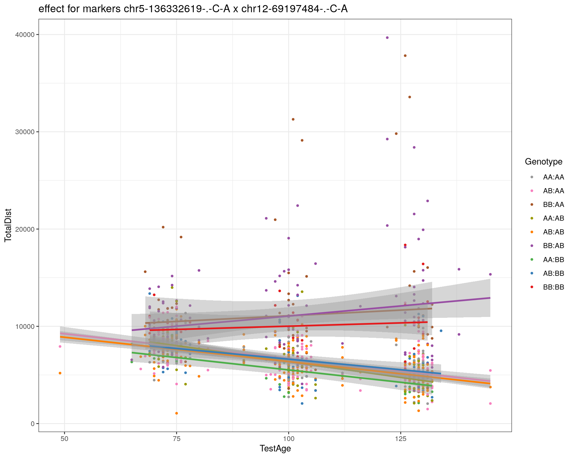

Past versions of “Plot the Dist_vs_age separate by genotype for each marker-117.png”

Version	Author	Date
2470aab	xhyuo	2022-12-24

Past versions of “Plot the Dist_vs_age separate by genotype for each marker-118.png”

Version	Author	Date
2470aab	xhyuo	2022-12-24

[1] "chr12-86851130-.-T-A"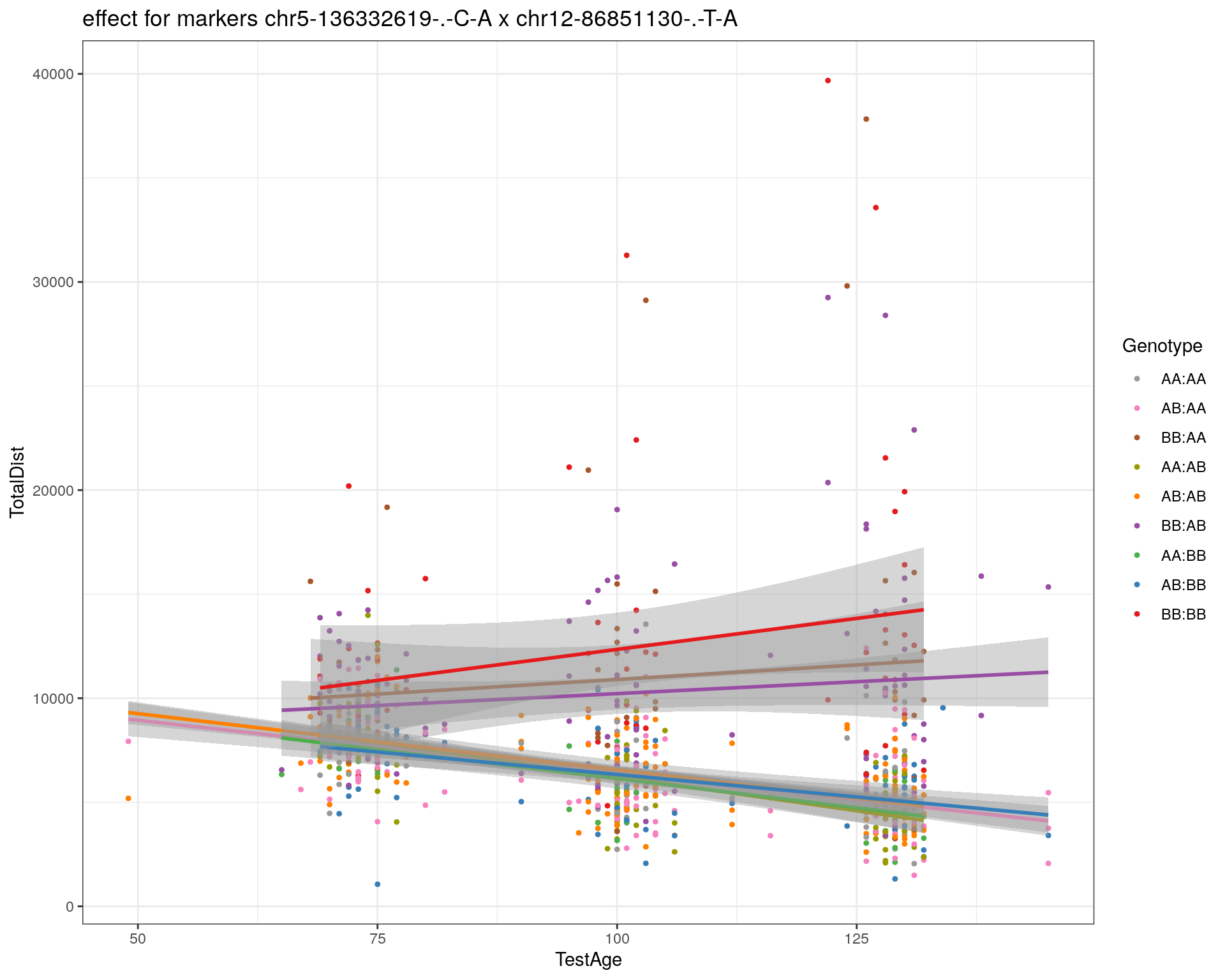

Past versions of “Plot the Dist_vs_age separate by genotype for each marker-119.png”

Version	Author	Date
2470aab	xhyuo	2022-12-24

Past versions of “Plot the Dist_vs_age separate by genotype for each marker-120.png”

Version	Author	Date
2470aab	xhyuo	2022-12-24

[1] "chr12-112415100-.-G-A"

Past versions of “Plot the Dist_vs_age separate by genotype for each marker-121.png”

Version	Author	Date
2470aab	xhyuo	2022-12-24

Past versions of “Plot the Dist_vs_age separate by genotype for each marker-122.png”

Version	Author	Date
2470aab	xhyuo	2022-12-24

[1] "chr13-20165684-.-T-A"

Past versions of “Plot the Dist_vs_age separate by genotype for each marker-123.png”

Version	Author	Date
2470aab	xhyuo	2022-12-24

Past versions of “Plot the Dist_vs_age separate by genotype for each marker-124.png”

Version	Author	Date
2470aab	xhyuo	2022-12-24

[1] "chr13-115031098-.-T-C"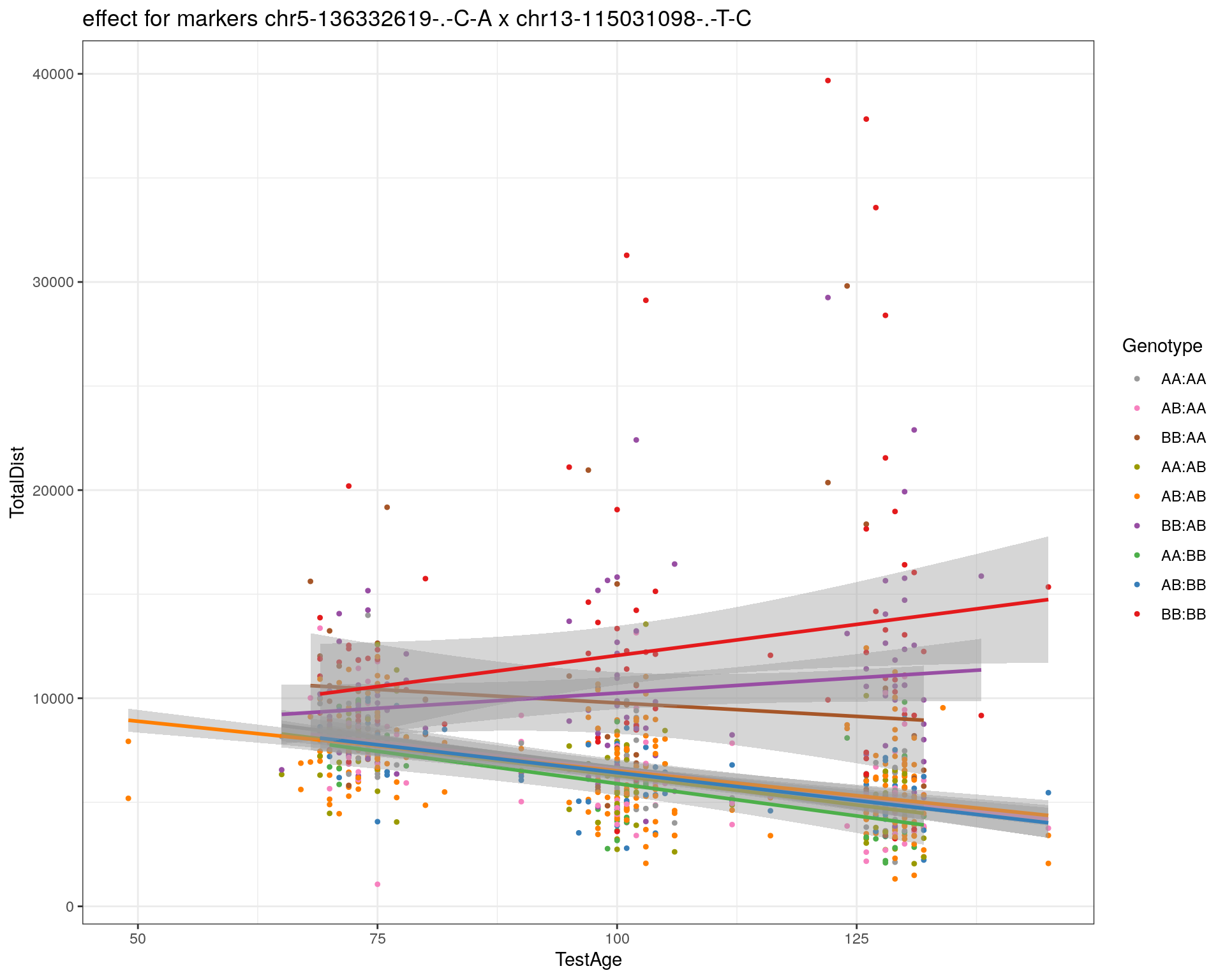

Past versions of “Plot the Dist_vs_age separate by genotype for each marker-125.png”

Version	Author	Date
2470aab	xhyuo	2022-12-24

Past versions of “Plot the Dist_vs_age separate by genotype for each marker-126.png”

Version	Author	Date
2470aab	xhyuo	2022-12-24

[1] "chr14-11709591-.-T-C"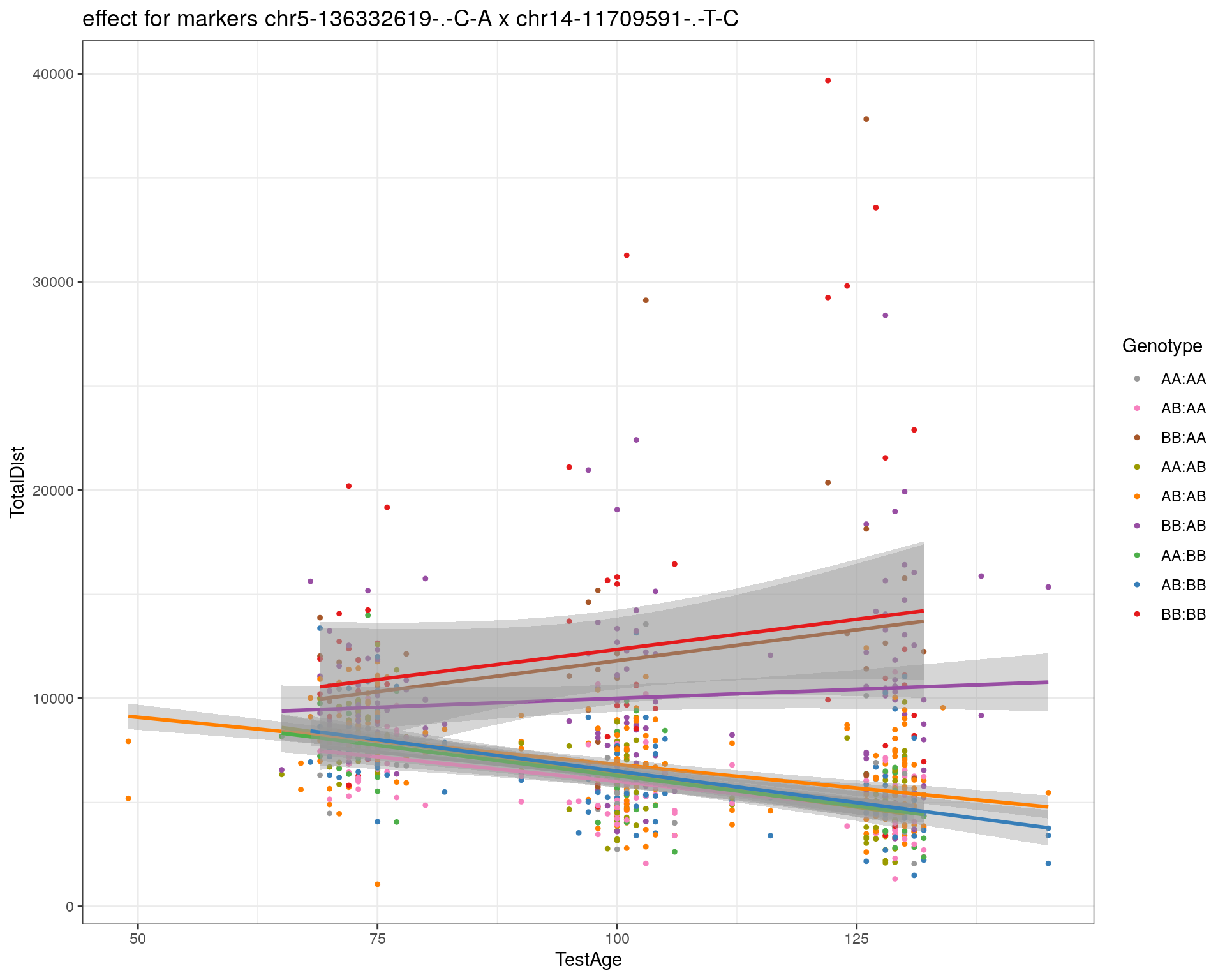

Past versions of “Plot the Dist_vs_age separate by genotype for each marker-127.png”

Version	Author	Date
2470aab	xhyuo	2022-12-24

Past versions of “Plot the Dist_vs_age separate by genotype for each marker-128.png”

Version	Author	Date
2470aab	xhyuo	2022-12-24

[1] "chr14-50642778-.-G-A"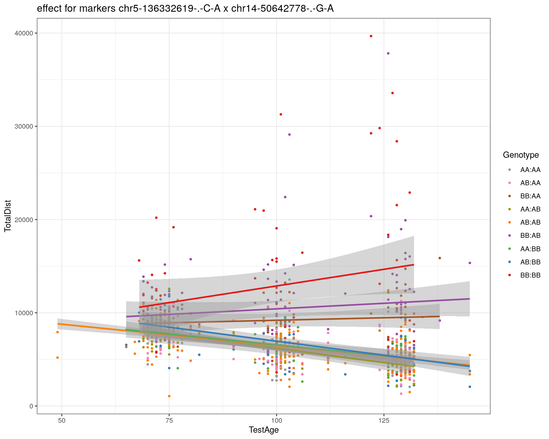

Past versions of “Plot the Dist_vs_age separate by genotype for each marker-129.png”

Version	Author	Date
2470aab	xhyuo	2022-12-24

Past versions of “Plot the Dist_vs_age separate by genotype for each marker-130.png”

Version	Author	Date
2470aab	xhyuo	2022-12-24

[1] "chr14-62407765-.-T-A"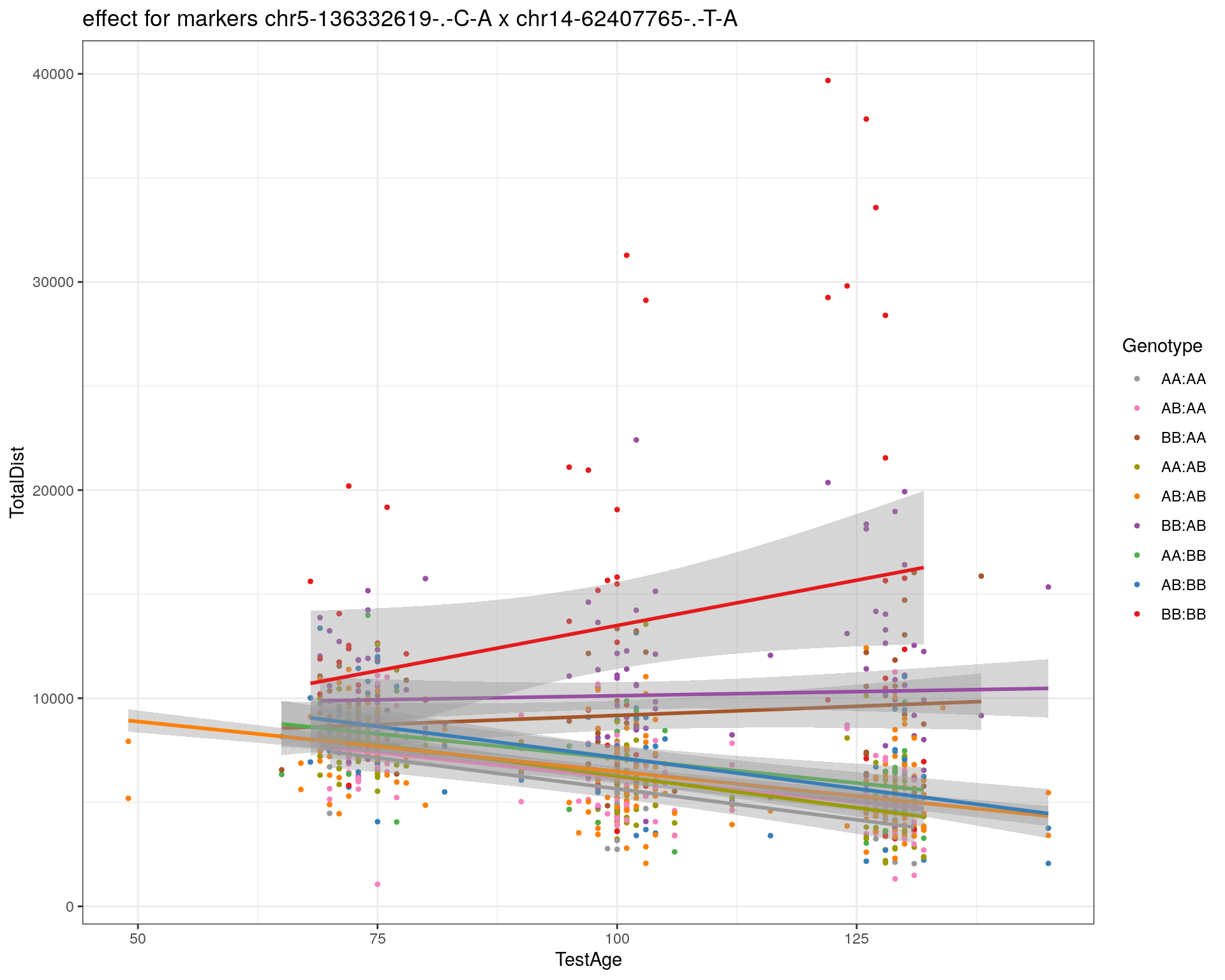

Past versions of “Plot the Dist_vs_age separate by genotype for each marker-131.png”

Version	Author	Date
2470aab	xhyuo	2022-12-24

Past versions of “Plot the Dist_vs_age separate by genotype for each marker-132.png”

Version	Author	Date
2470aab	xhyuo	2022-12-24

[1] "chr14-69691477-.-G-T"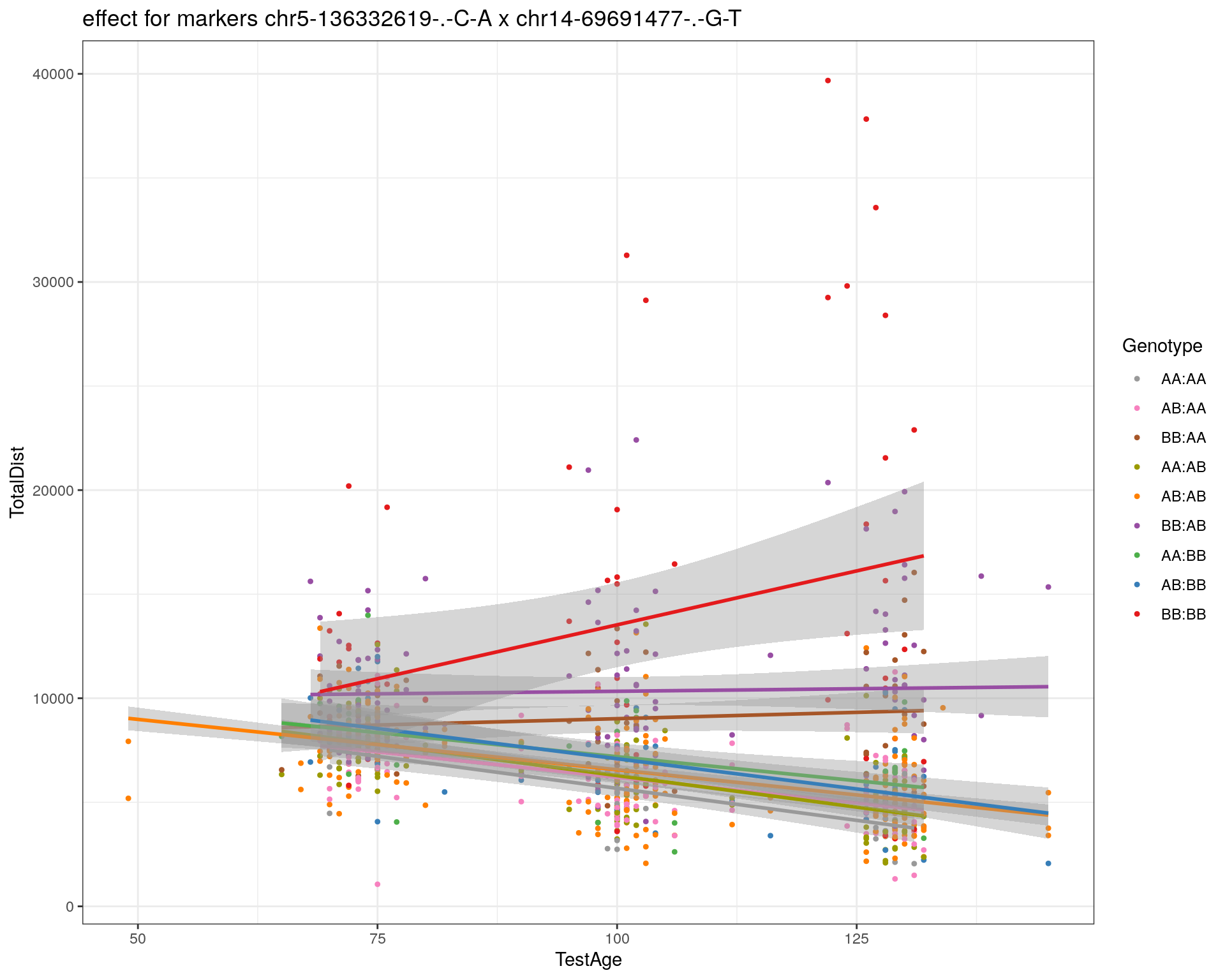

Past versions of “Plot the Dist_vs_age separate by genotype for each marker-133.png”

Version	Author	Date
2470aab	xhyuo	2022-12-24

Past versions of “Plot the Dist_vs_age separate by genotype for each marker-134.png”

Version	Author	Date
2470aab	xhyuo	2022-12-24

[1] "chr15-58605950-.-C-G"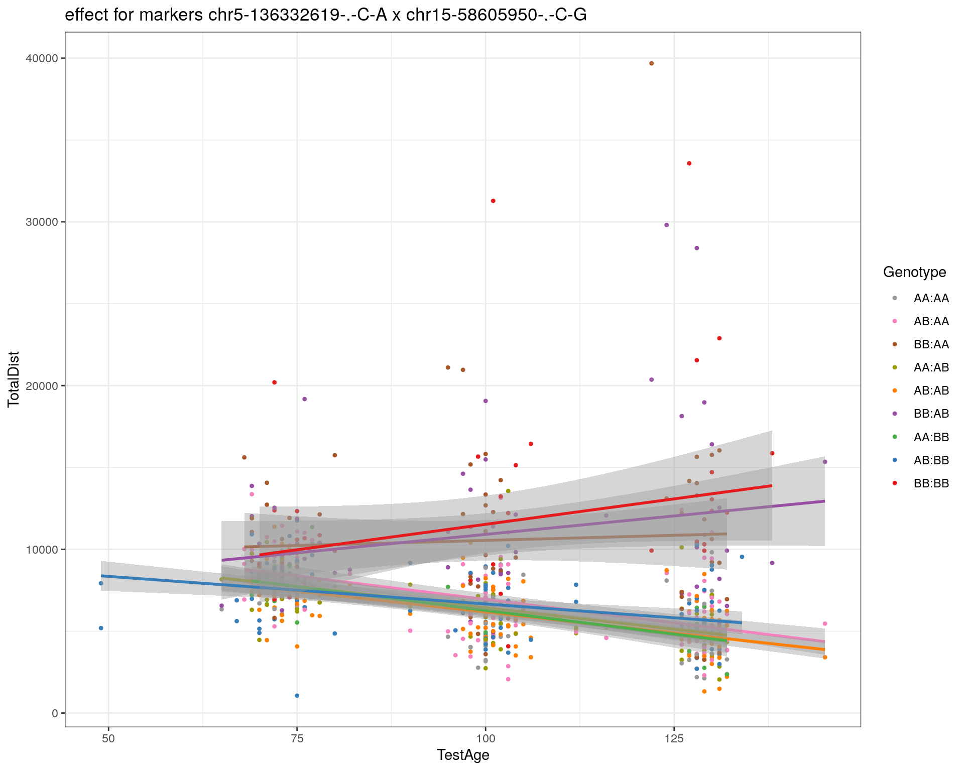

Past versions of “Plot the Dist_vs_age separate by genotype for each marker-135.png”

Version	Author	Date
2470aab	xhyuo	2022-12-24

Past versions of “Plot the Dist_vs_age separate by genotype for each marker-136.png”

Version	Author	Date
2470aab	xhyuo	2022-12-24

[1] "chr15-74727869-.-C-T"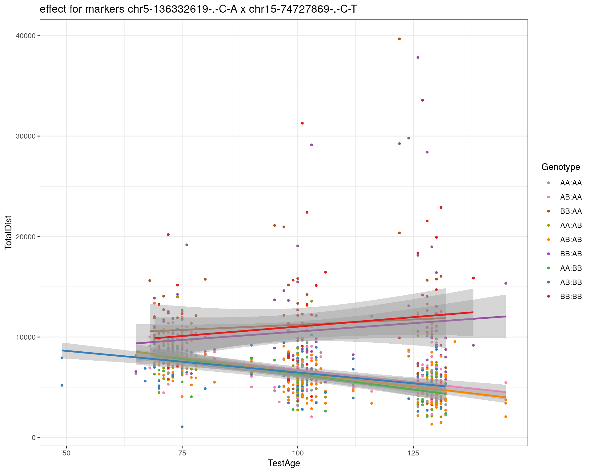

Past versions of “Plot the Dist_vs_age separate by genotype for each marker-137.png”

Version	Author	Date
2470aab	xhyuo	2022-12-24

Past versions of “Plot the Dist_vs_age separate by genotype for each marker-138.png”

Version	Author	Date
2470aab	xhyuo	2022-12-24

[1] "chr16-32593683-.-A-G"

Past versions of “Plot the Dist_vs_age separate by genotype for each marker-139.png”

Version	Author	Date
2470aab	xhyuo	2022-12-24

Past versions of “Plot the Dist_vs_age separate by genotype for each marker-140.png”

Version	Author	Date
2470aab	xhyuo	2022-12-24

[1] "chr16-75648687-.-G-A"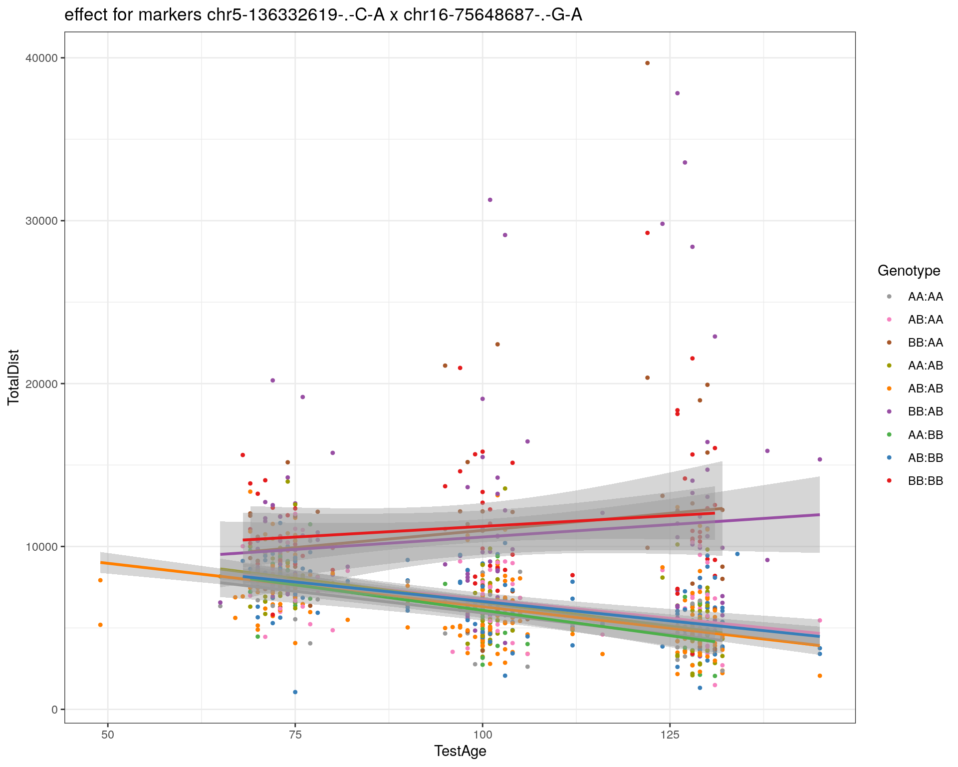

Past versions of “Plot the Dist_vs_age separate by genotype for each marker-141.png”

Version	Author	Date
2470aab	xhyuo	2022-12-24

Past versions of “Plot the Dist_vs_age separate by genotype for each marker-142.png”

Version	Author	Date
2470aab	xhyuo	2022-12-24

[1] "chr17-61305603-.-G-A"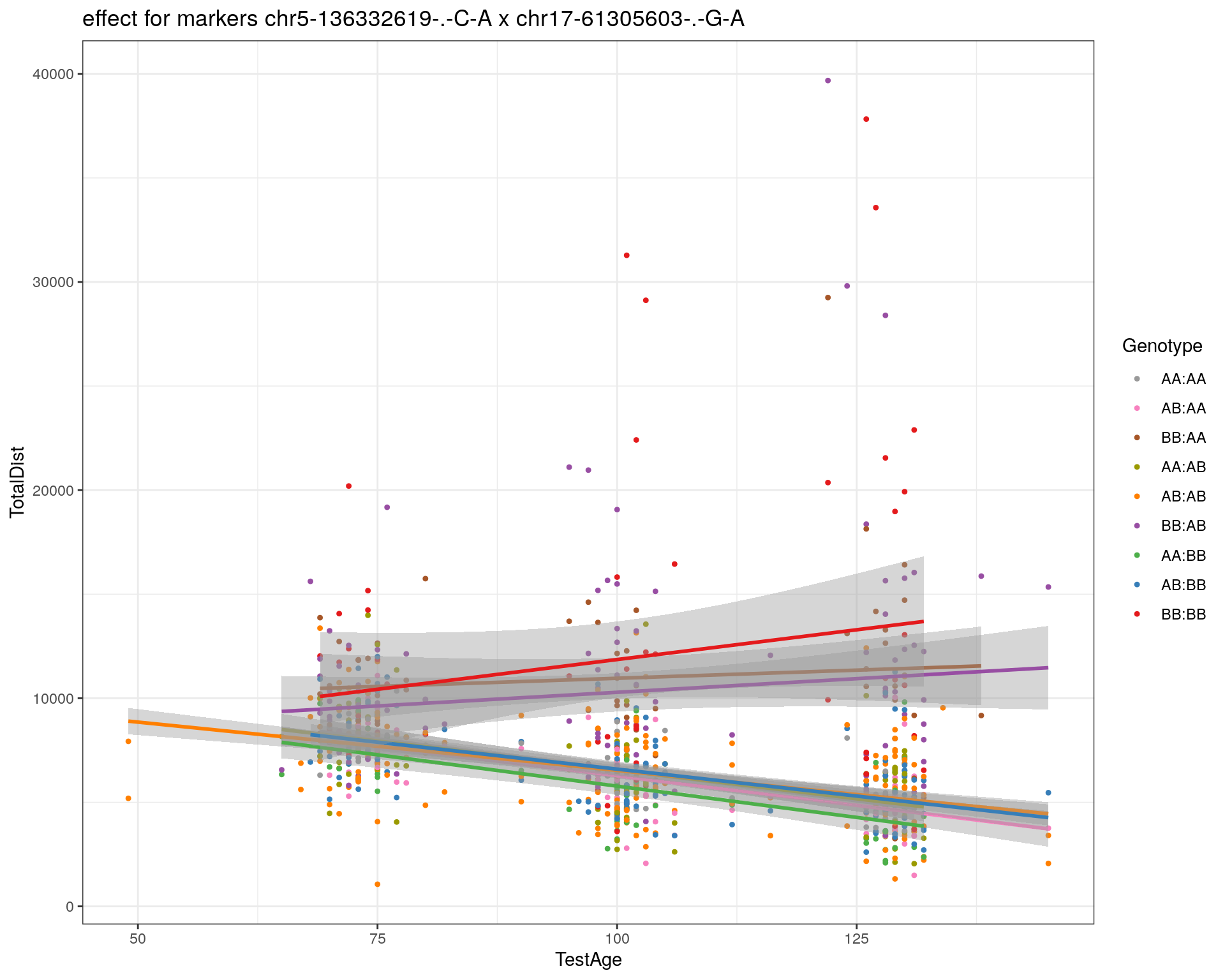

Past versions of “Plot the Dist_vs_age separate by genotype for each marker-143.png”

Version	Author	Date
2470aab	xhyuo	2022-12-24

Past versions of “Plot the Dist_vs_age separate by genotype for each marker-144.png”

Version	Author	Date
2470aab	xhyuo	2022-12-24

[1] "chr17-69219676-.-G-A"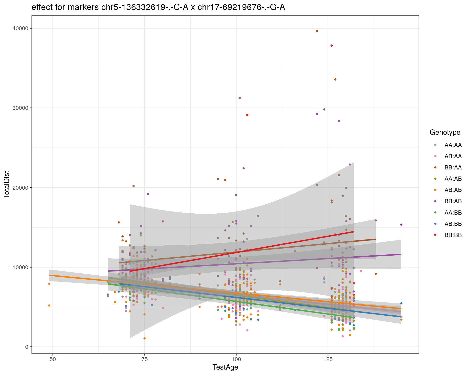

Past versions of “Plot the Dist_vs_age separate by genotype for each marker-145.png”

Version	Author	Date
2470aab	xhyuo	2022-12-24

Past versions of “Plot the Dist_vs_age separate by genotype for each marker-146.png”

Version	Author	Date
2470aab	xhyuo	2022-12-24

[1] "chr18-51300216-.-T-A"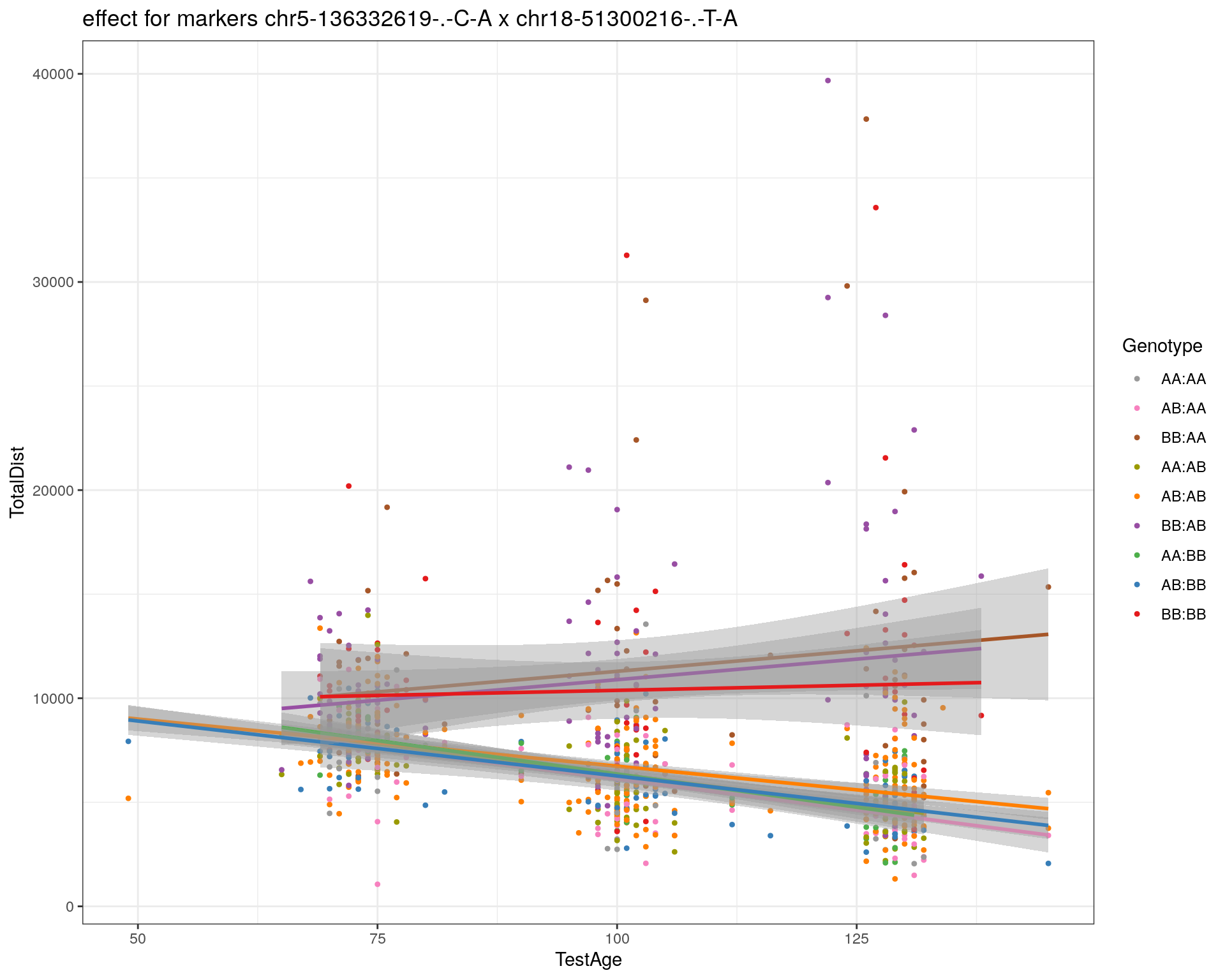

Past versions of “Plot the Dist_vs_age separate by genotype for each marker-147.png”

Version	Author	Date
2470aab	xhyuo	2022-12-24

Past versions of “Plot the Dist_vs_age separate by genotype for each marker-148.png”

Version	Author	Date
2470aab	xhyuo	2022-12-24

[1] "chr18-89347666-.-A-G"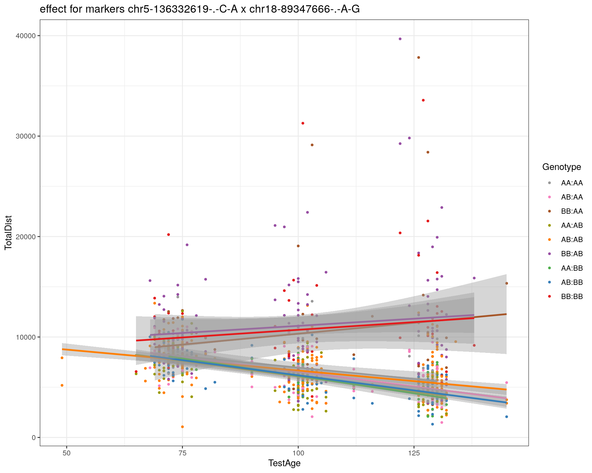

Past versions of “Plot the Dist_vs_age separate by genotype for each marker-149.png”

Version	Author	Date
2470aab	xhyuo	2022-12-24

Past versions of “Plot the Dist_vs_age separate by genotype for each marker-150.png”

Version	Author	Date
2470aab	xhyuo	2022-12-24

[1] "chr19-29815794-.-A-T"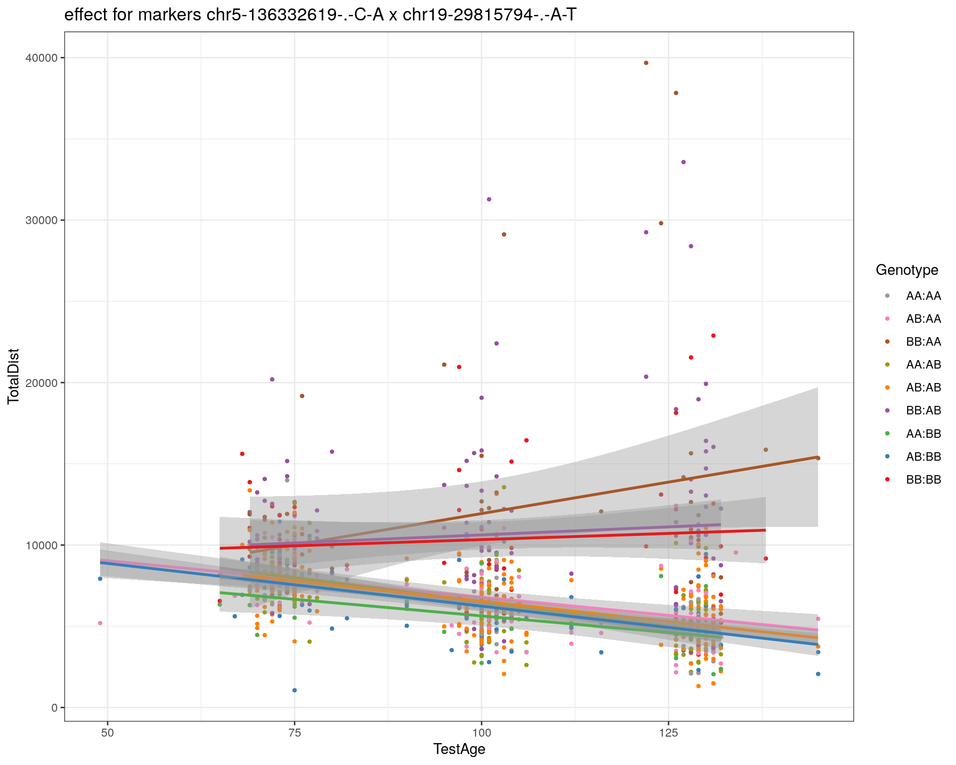

Past versions of “Plot the Dist_vs_age separate by genotype for each marker-151.png”

Version	Author	Date
2470aab	xhyuo	2022-12-24

Past versions of “Plot the Dist_vs_age separate by genotype for each marker-152.png”

Version	Author	Date
2470aab	xhyuo	2022-12-24

[1] "chr19-45958839-.-A-T"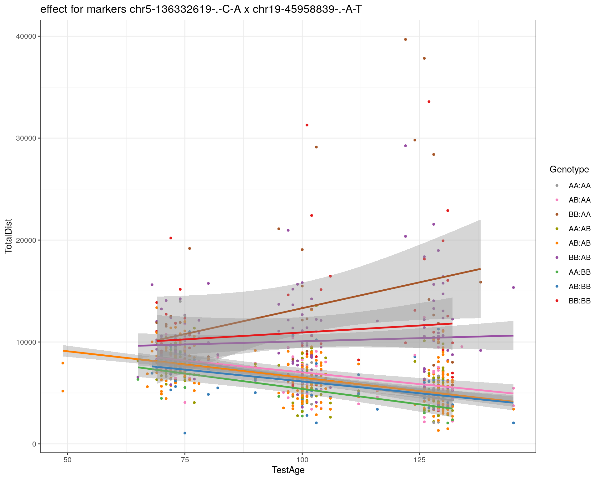

Past versions of “Plot the Dist_vs_age separate by genotype for each marker-153.png”

Version	Author	Date
2470aab	xhyuo	2022-12-24

Past versions of “Plot the Dist_vs_age separate by genotype for each marker-154.png”

Version	Author	Date
2470aab	xhyuo	2022-12-24

[1] "chr19-53469239-.-A-G"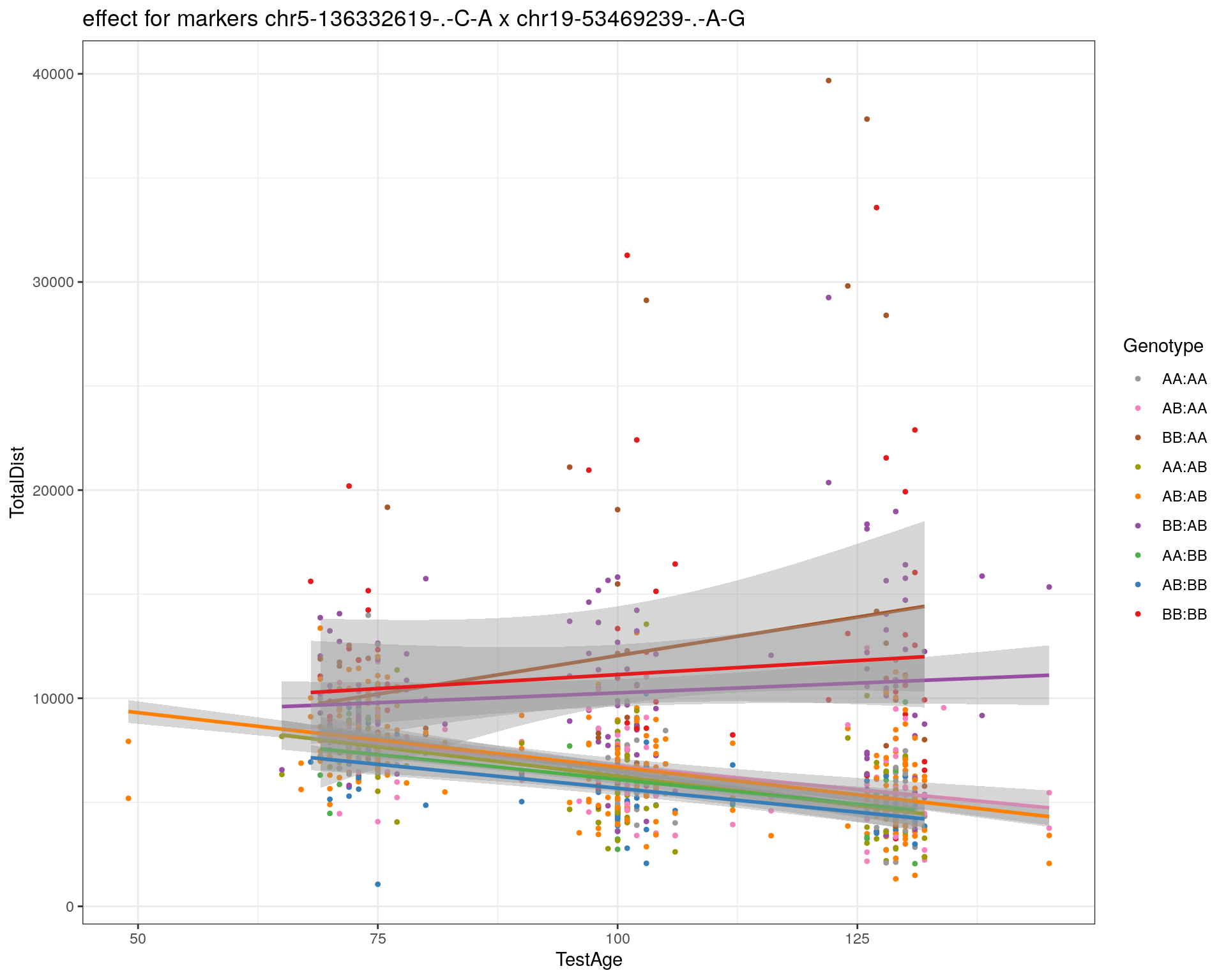

Past versions of “Plot the Dist_vs_age separate by genotype for each marker-155.png”

Version	Author	Date
2470aab	xhyuo	2022-12-24

Past versions of “Plot the Dist_vs_age separate by genotype for each marker-156.png”

Version	Author	Date
2470aab	xhyuo	2022-12-24

pdf(paste0("output/", paste0("WT144_effect_for_marker_", "_int_chr5-136332619-.-C-A"), ".pdf"))
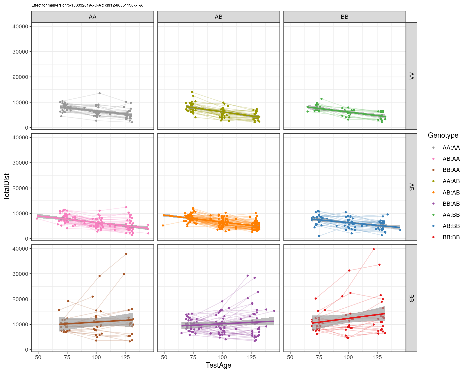
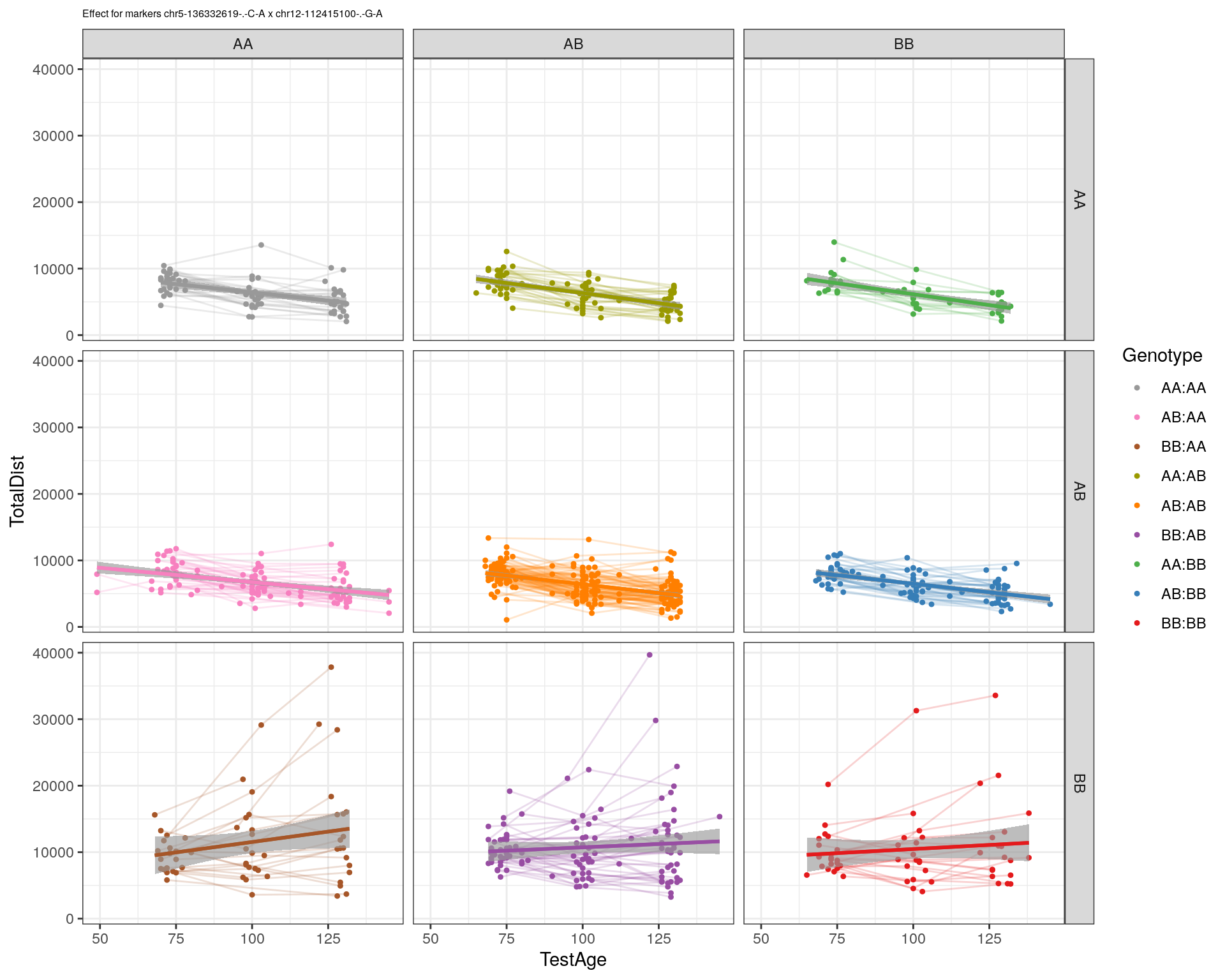
plot_int_graph(WT144, paste0("WT144_effect_for_marker_", "_int_chr5-136332619-.-C-A"), "chr5-136332619-.-C-A")

[1] "chr1-65643621-.-C-A"

[1] "chr1-74679418-.-A-G"

[1] "chr1-79823528-.-A-G"

[1] "chr1-86851039-.-A-G"

[1] "chr1-188155143-.-G-A"

[1] "chr2-7018694-.-G-T"

[1] "chr2-79706301-.-T-A"

[1] "chr2-92367783-.-T-C"

[1] "chr2-95118744-.-T-A"

[1] "chr2-102169266-.-C-T"

[1] "chr2-130405980-.-A-T"

[1] "chr2-137498061-.-T-A"

[1] "chr2-145128463-.-A-T"

[1] "chr3-59218564-.-T-A"

[1] "chr3-98881230-.-G-A"

[1] "chr3-106985708-.-A-C"

[1] "chr3-135614002-.-T-G"

[1] "chr3-145286160-.-C-A"

[1] "chr3-146750531-.-A-G"

[1] "chr3-152699551-.-G-A"

[1] "chr4-32821418-.-C-T"

[1] "chr5-75264187-.-T-C"

[1] "chr5-90233933-.-A-T"

[1] "chr5-97607237-.-T-A"

[1] "chr5-107507008-.-C-T"

[1] "chr5-112799362-.-C-T"

[1] "chr5-120660771-.-T-A"

[1] "chr5-122167749-.-T-C"

[1] "chr5-125153901-.-C-T"

[1] "chr5-126058493-.-T-A"

[1] "chr5-126551890-.-T-A"

[1] "chr5-127565504-.-T-A"

[1] "chr5-130394596-.-T-C"

[1] "chr5-130943677-.-T-A"

[1] "chr5-131298836-.-T-C"

[1] "chr5-133052642-.-T-G"

[1] "chr5-135960983-.-T-C"

[1] "chr5-136332619-.-C-A"

[1] "chr5-136844385-.-T-G"

[1] "chr5-138956439-.-T-C"

[1] "chr5-139706036-.-T-C"

[1] "chr5-139891407-.-T-C"

[1] "chr5-140071081-.-C-A"

[1] "chr7-35061547-.-A-G"

[1] "chr7-44272713-.-T-C"

[1] "chr7-66785411-.-A-G"

[1] "chr7-112510032-.-A-T"

[1] "chr8-91986173-.-T-C"

[1] "chr8-99395759-.-T-C"

[1] "chr8-112465004-.-G-A"

[1] "chr9-64698947-.-C-T"

[1] "chr9-65857475-.-T-C"

[1] "chr9-69415567-.-T-A"

[1] "chr9-71739608-.-T-A"

[1] "chr9-80465702-.-T-A"

[1] "chr10-24134777-.-A-T"

[1] "chr11-96730656-.-A-G"

[1] "chr12-43136399-.-A-T"

[1] "chr12-69197484-.-C-A"

[1] "chr12-86851130-.-T-A"

[1] "chr12-112415100-.-G-A"

[1] "chr13-20165684-.-T-A"

[1] "chr13-115031098-.-T-C"

[1] "chr14-11709591-.-T-C"

[1] "chr14-50642778-.-G-A"

[1] "chr14-62407765-.-T-A"

[1] "chr14-69691477-.-G-T"

[1] "chr15-58605950-.-C-G"

[1] "chr15-74727869-.-C-T"

[1] "chr16-32593683-.-A-G"

[1] "chr16-75648687-.-G-A"

[1] "chr17-61305603-.-G-A"

[1] "chr17-69219676-.-G-A"

[1] "chr18-51300216-.-T-A"

[1] "chr18-89347666-.-A-G"

[1] "chr19-29815794-.-A-T"

[1] "chr19-45958839-.-A-T"

[1] "chr19-53469239-.-A-G"

dev.off()

png 
  2 

Figure panel for publication

# define a function that emits the desired plot
figA <- function() {
  par(
    mar = c(3, 5, 1, 1),
    mgp = c(2, 1, 0)
  )
  #plot phenotypes: slope and totaldistance3
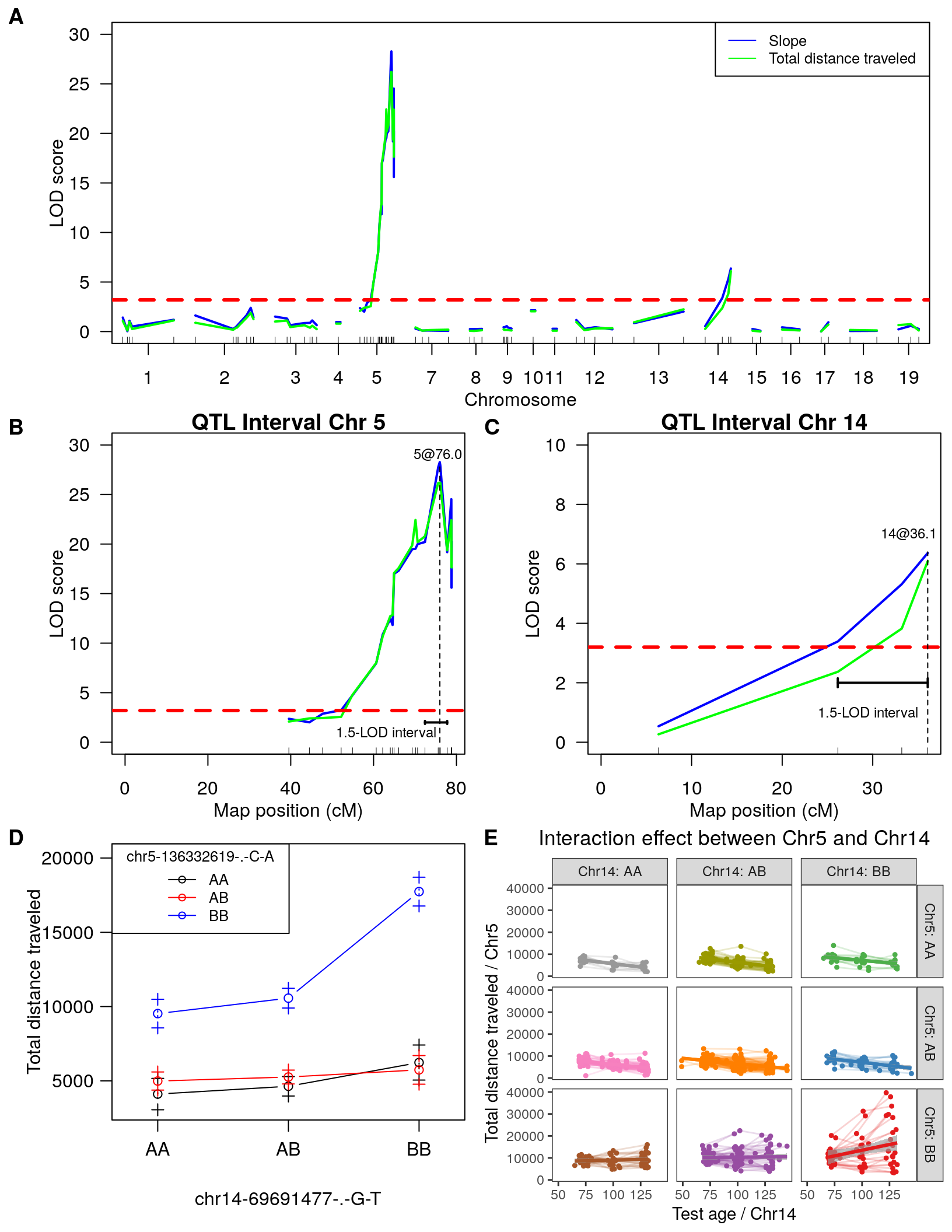
  plot(out.mr[[2]], col= "blue", ylim = c(0, 30), ylab = "LOD score")
  plot(out.mr[[1]], col=  "green", add=TRUE)
  abline(h=3.2, col="red", lty=2, lwd=3)
  # Add a legend
  legend("topright", 
         legend=c("Slope", "Total distance traveled"),
         col=c("blue", "green"), lty=1, cex=0.8)
}

figB <- function() {
  par(
    mar = c(3, 5, 1, 0.5),
    mgp = c(2, 1, 0)
  )
  #only at chr 5 and 14
  #plot phenotypes: slope and totaldistance3
  plot(out.mr[[2]], col= "blue", ylim = c(0, 30), ylab = "LOD score", chr = c(5), main = "QTL Interval Chr 5")
  plot(out.mr[[1]], col=  "green", add=TRUE, chr = c(5))
  abline(h=3.2, col="red", lty=2, lwd=3)
  #abline(v= 76.0, col="black", lty=2, lwd=1)
  text(75.5, 29, "5@76.0", cex = 0.75)
  segments(x0 = 76,
         x1 = 76,
         y0 = 0,
         y1 = 28,
         col="black", lty=2, lwd=1)
    segments(x0 = 72.40574,
         x1 = 77.76853,
         y0 = 2,
         y1 = 2,
         col="black", lty=1, lwd=2)
    segments(x0 = 72.40574,
         x1 = 72.40574,
         y0 = 1.85,
         y1 = 2.15,
         col="black", lty=1, lwd=2)
    segments(x0 = 77.76853,
         x1 = 77.76853,
         y0 = 1.85,
         y1 = 2.15,
         col="black", lty=1, lwd=2)
    text(63, 1, "1.5-LOD interval", cex = 0.75)
  # Add a legend
  # legend("topright", 
  #        legend=c("Slope", "Total Distance traveled"),
  #        col=c("blue", "green"), lty=1, cex=0.8)
}


figC <- function() {
  par(
    mar = c(3, 5, 1, 0.5),
    mgp = c(2, 1, 0)
  )
  #only at chr 5 and 14
  #plot phenotypes: slope and totaldistance3
plot(out.mr[[2]], col= "blue", ylim = c(0, 10), ylab = "LOD score", chr = c(14), main = "QTL Interval Chr 14")
plot(out.mr[[1]], col=  "green", add=TRUE, chr = c(14))
abline(h=3.2, col="red", lty=2, lwd=3)
#abline(v= 76.0, col="black", lty=2, lwd=1)
text(34, 7, "14@36.1", cex = 0.75)
segments(x0 = 36.07219,
         x1 = 36.07219,
         y0 = 0,
         y1 = 6.4,
         col="black", lty=2, lwd=1)
segments(x0 = 26.14,
         x1 = 36.07219,
         y0 = 2,
         y1 = 2,
         col="black", lty=1, lwd=2)
segments(x0 = 26.14,
         x1 = 26.14,
         y0 = 1.85,
         y1 = 2.15,
         col="black", lty=1, lwd=2)
segments(x0 = 36.07219,
         x1 = 36.07219,
         y0 = 1.85,
         y1 = 2.15,
         col="black", lty=1, lwd=2)
text(29.5, 1, "1.5-LOD interval", cex = 0.75)
  # Add a legend
  # legend("topright", 
  #        legend=c("Slope", "Total Distance traveled"),
  #        col=c("blue", "green"), lty=1, cex=0.8)
}


figD <- function() {
 par(mar = c(5, 5, 1, 0.5), 
     mgp = c(3, 0.8, 0))
  #interaction_effect for slope
  effectplot(WT144, main = "",
             mname1 = marker[[1]], 
             mname2 = marker[[2]], ylab = "Total distance traveled", 
             xlab = marker[[2]],
             pheno.col = 11, add.legend=F)
  # Add a legend
  legend("topleft", legend=c("AA", "AB", "BB"), title = marker[[1]],
       col=c("black","red", "blue"), pch = 1, lty=1, cex=0.8)
}

figE <- function() {
  par(
    mar = c(3, 5, 1, 1),
    mgp = c(3, 1, 0)
  )
  #interaction_effect for slope
  effectplot(WT144, main = "",
             mname1 = marker[[1]], 
             mname2 = marker[[2]], ylab = "Slope",xlab = marker[[2]],
             pheno.col = 15, add.legend=F)
}

cross = WT144
basem = "chr5-136332619-.-C-A"

# Plot the Dist vs age, separate by genotype for each marker
allphen <- cross$pheno
allgeno <- as.data.frame(pull.geno(cross))
rownames(allgeno) <- cross$pheno$AnimalName
allphen <- merge(allphen, allgeno, by.x="AnimalName", by.y="row.names", all.x=TRUE)
#pdf(paste0("output/", name, ".pdf"))
#for (mar in colnames(allgeno)){
mar = "chr14-69691477-.-G-T"
  print(mar)

[1] "chr14-69691477-.-G-T"

  subplot <- allphen[!is.na(allphen[,mar, drop=FALSE]),] %>% 
    pivot_longer(cols = starts_with("TestAge_"), names_to="test.no", values_to = "Age") %>% 
    separate(test.no, c("empty1", "test1")) %>%
    pivot_longer(cols = starts_with("TotalDist_"), names_to="test.no.2", values_to = "Dist") %>%
    separate(test.no.2, c("empty2", "test2")) %>% filter(test1==test2)
  subplot <- as.data.frame(subplot)
  subplot$interactions <- factor(subplot[, basem] + subplot[, mar]*3)
  # 1:1 -> 4 1:2 -> 7 1:3 -> 10
  # 2:1 -> 5 2:2 -> 8 2:3 -> 11
  # 3:1 -> 6 3:2 -> 9 3:3 -> 12
  itypes  <- c(1,2,3,"AA:AA", "AB:AA", "BB:AA", 
               "AA:AB", "AB:AB", "BB:AB",
               "AA:BB", "AB:BB", "BB:BB")
  levels(subplot$interactions) <- itypes[as.integer(levels(subplot$interactions))]
  
  #replaces 1 2 and 3 as AA, AB and BB
  subplot[, basem][subplot[, basem] == 1] <- "AA"
  subplot[, basem][subplot[, basem] == 2] <- "AB"
  subplot[, basem][subplot[, basem] == 3] <- "BB"
  subplot[, mar][subplot[, mar] == 1] <- "AA"
  subplot[, mar][subplot[, mar] == 2] <- "AB"
  subplot[, mar][subplot[, mar] == 3] <- "BB"
  
  p1 <- ggplot(subplot, aes(Age, Dist, color=interactions, group=interactions)) + 
    geom_point(shape = 20, size=0.75) + 
    #scale_color_discrete("Genotype") +
    labs(color = "Genotype") +
    ylab("TotalDist") +
    xlab("Test Age") +
    #scale_color_brewer(palette = "Set1") + 
    scale_color_manual(breaks = c("AA:AA", "AB:AA", "BB:AA", "AA:AB",
                                  "AB:AB", "BB:AB", "AA:BB", "AB:BB", "BB:BB"),
                       #values = RColorBrewer::brewer.pal(9, "Set1")[9:1]) +
                       values = c("#999999", "#F781BF", "#A65628","#9a9a00", "#FF7F00", "#984EA3", "#4DAF4A", "#377EB8", "#E41A1C")) +
    stat_smooth(method="lm", show.legend = FALSE, formula = y~x) + 
    labs(title=paste0("effect for markers ", basem, " x ", mar)) +
    theme_bw()
  print(p1)

Warning: Removed 29 rows containing non-finite values (stat_smooth).

Warning: Removed 29 rows containing missing values (geom_point).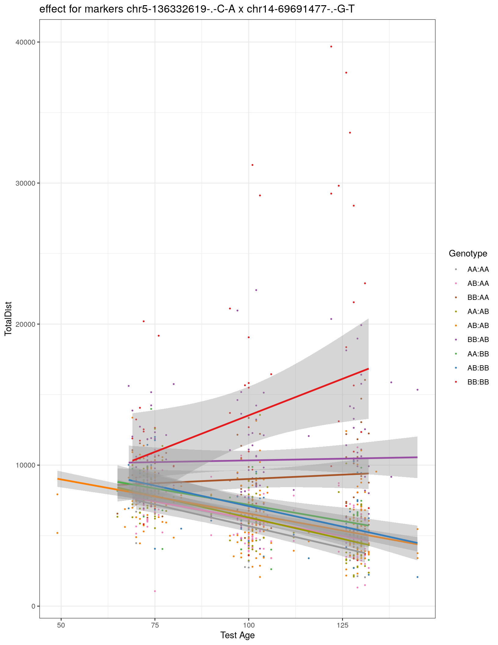

Past versions of “Figure panel for publication-1.png”

Version	Author	Date
2470aab	xhyuo	2022-12-24

  colnames(subplot)[colnames(subplot) == basem] = "Chr5"
  colnames(subplot)[colnames(subplot) == mar] = "Chr14"
  p2 <- ggplot(subplot, aes(Age, Dist, color=interactions, group=interactions)) +
    geom_point(shape = 20, show.legend = FALSE) +
    geom_line(aes(group = AnimalName, color = interactions), show.legend = FALSE, alpha = 0.2) +  
    geom_smooth(method='lm', formula= y~x, show.legend = FALSE, size = 1) +
    #scale_color_discrete("Genotype") +
    labs(color = "Genotype") +
    ylab("Total distance traveled / Chr5") +
    xlab("Test age / Chr14") +
    #scale_color_brewer(palette = "Set1") + 
    scale_color_manual(breaks = c("AA:AA", "AB:AA", "BB:AA", "AA:AB",
                                  "AB:AB", "BB:AB", "AA:BB", "AB:BB", "BB:BB"),
                       #values = RColorBrewer::brewer.pal(9, "Set1")[9:1]) +
                       values = c("#999999", "#F781BF", "#A65628","#9a9a00", "#FF7F00", "#984EA3", "#4DAF4A", "#377EB8", "#E41A1C")) +
    stat_smooth(method="lm", show.legend = FALSE, formula = y~x) + 
    labs(title=paste0("Interaction effect between Chr5 and Chr14")) +
    facet_grid(rows = vars(Chr5), cols = vars(Chr14), labeller = label_both) +
    theme_bw() +
    theme(panel.grid.major = element_blank(), panel.grid.minor = element_blank()) +
    theme(plot.title = element_text(hjust = 0.5))
  print(p2)

Warning: Removed 29 rows containing non-finite values (stat_smooth).

Warning: Removed 29 rows containing non-finite values (stat_smooth).

Warning: Removed 29 rows containing missing values (geom_point).

Warning: Removed 29 row(s) containing missing values (geom_path).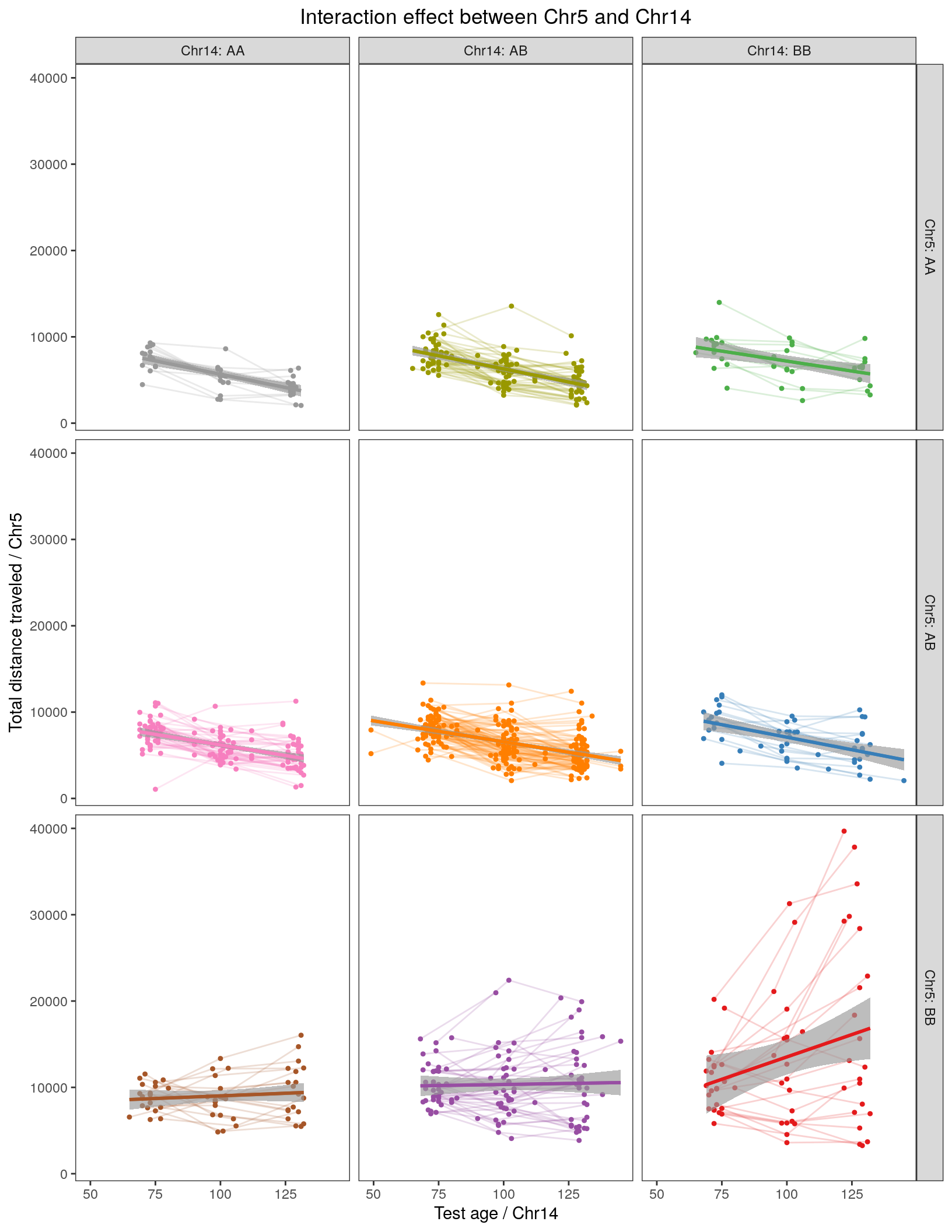

Past versions of “Figure panel for publication-2.png”

Version	Author	Date
2470aab	xhyuo	2022-12-24

pp2 = plot_grid(figB, figC, labels = c("B", "C"), align = 'h', ncol=2)
pp3 = plot_grid(figD, p2, labels = c("D", "E"), align = 'h',ncol=2)

Warning: Removed 29 rows containing non-finite values (stat_smooth).

Warning: Removed 29 rows containing non-finite values (stat_smooth).

Warning: Removed 29 rows containing missing values (geom_point).

Warning: Removed 29 row(s) containing missing values (geom_path).

Warning: Graphs cannot be horizontally aligned unless the axis parameter is set.
Placing graphs unaligned.

pdf("output/figure_panel.pdf", width = 8.5, height = 11)
plot_grid(figA, labels = c('A', ''),
  pp2,
  pp3,
  nrow = 3
)
dev.off()

png 
  2 

plot_grid(figA, labels = c('A', ''),
  pp2,
  pp3,
  nrow = 3
)

Past versions of “Figure panel for publication-3.png”

Version	Author	Date
2470aab	xhyuo	2022-12-24

Session information

sessionInfo()

R version 4.0.3 (2020-10-10)
Platform: x86_64-pc-linux-gnu (64-bit)
Running under: Ubuntu 20.04.2 LTS

Matrix products: default
BLAS/LAPACK: /usr/lib/x86_64-linux-gnu/openblas-pthread/libopenblasp-r0.3.8.so

locale:
 [1] LC_CTYPE=en_US.UTF-8       LC_NUMERIC=C              
 [3] LC_TIME=en_US.UTF-8        LC_COLLATE=en_US.UTF-8    
 [5] LC_MONETARY=en_US.UTF-8    LC_MESSAGES=C             
 [7] LC_PAPER=en_US.UTF-8       LC_NAME=C                 
 [9] LC_ADDRESS=C               LC_TELEPHONE=C            
[11] LC_MEASUREMENT=en_US.UTF-8 LC_IDENTIFICATION=C       

attached base packages:
[1] stats     graphics  grDevices utils     datasets  methods   base     

other attached packages:
 [1] cowplot_1.1.1     qtl2_0.24         lmerTest_3.1-3    lme4_1.1-26      
 [5] Matrix_1.3-2      forcats_0.5.1     stringr_1.4.0     dplyr_1.0.4      
 [9] purrr_0.3.4       readr_1.4.0       tidyr_1.1.2       tibble_3.0.6     
[13] tidyverse_1.3.0   qtlcharts_0.12-10 qtl_1.47-9        gridExtra_2.3    
[17] ggplot2_3.3.3     workflowr_1.6.2  

loaded via a namespace (and not attached):
 [1] nlme_3.1-152        fs_1.5.0            lubridate_1.7.9.2  
 [4] bit64_4.0.5         RColorBrewer_1.1-2  httr_1.4.2         
 [7] rprojroot_2.0.2     numDeriv_2016.8-1.1 tools_4.0.3        
[10] backports_1.2.1     R6_2.5.0            mgcv_1.8-34        
[13] DBI_1.1.1           colorspace_2.0-0    withr_2.4.1        
[16] tidyselect_1.1.0    bit_4.0.4           compiler_4.0.3     
[19] git2r_0.28.0        cli_2.3.0           rvest_0.3.6        
[22] xml2_1.3.2          labeling_0.4.2      scales_1.1.1       
[25] digest_0.6.27       minqa_1.2.4         rmarkdown_2.6      
[28] pkgconfig_2.0.3     htmltools_0.5.1.1   highr_0.8          
[31] dbplyr_2.1.0        fastmap_1.1.0       rlang_1.0.2        
[34] readxl_1.3.1        rstudioapi_0.13     RSQLite_2.2.3      
[37] gridGraphics_0.5-1  farver_2.0.3        generics_0.1.0     
[40] jsonlite_1.7.2      magrittr_2.0.1      Rcpp_1.0.6         
[43] munsell_0.5.0       lifecycle_1.0.0     stringi_1.5.3      
[46] whisker_0.4         yaml_2.2.1          MASS_7.3-53.1      
[49] grid_4.0.3          blob_1.2.1          parallel_4.0.3     
[52] promises_1.2.0.1    crayon_1.4.1        lattice_0.20-41    
[55] haven_2.3.1         splines_4.0.3       hms_1.0.0          
[58] knitr_1.31          pillar_1.4.7        boot_1.3-27        
[61] reprex_1.0.0        glue_1.4.2          evaluate_0.14      
[64] data.table_1.13.6   modelr_0.1.8        vctrs_0.3.6        
[67] nloptr_1.2.2.2      httpuv_1.5.5        cellranger_1.1.0   
[70] gtable_0.3.0        assertthat_0.2.1    cachem_1.0.4       
[73] xfun_0.21           broom_0.7.4         later_1.1.0.1      
[76] memoise_2.0.0       statmod_1.4.35      ellipsis_0.3.1