Variant_plot
Hao He
Last updated: 2023-04-25
Checks: 7 0
Knit directory: QTL_analysis_for_Crichton/
This reproducible R Markdown analysis was created with workflowr (version 1.6.2). The Checks tab describes the reproducibility checks that were applied when the results were created. The Past versions tab lists the development history.
Great! Since the R Markdown file has been committed to the Git repository, you know the exact version of the code that produced these results.
Great job! The global environment was empty. Objects defined in the global environment can affect the analysis in your R Markdown file in unknown ways. For reproduciblity it’s best to always run the code in an empty environment.
The command set.seed(20221224) was run prior to running the code in the R Markdown file. Setting a seed ensures that any results that rely on randomness, e.g. subsampling or permutations, are reproducible.
Great job! Recording the operating system, R version, and package versions is critical for reproducibility.
Nice! There were no cached chunks for this analysis, so you can be confident that you successfully produced the results during this run.
Great job! Using relative paths to the files within your workflowr project makes it easier to run your code on other machines.
Great! You are using Git for version control. Tracking code development and connecting the code version to the results is critical for reproducibility.
The results in this page were generated with repository version 41e9673. See the Past versions tab to see a history of the changes made to the R Markdown and HTML files.
Note that you need to be careful to ensure that all relevant files for the analysis have been committed to Git prior to generating the results (you can use wflow_publish or wflow_git_commit). workflowr only checks the R Markdown file, but you know if there are other scripts or data files that it depends on. Below is the status of the Git repository when the results were generated:
Ignored files:
    Ignored:    .Rhistory
    Ignored:    .Rproj.user/

Untracked files:
    Untracked:  analysis/plot.R
    Untracked:  data/vcf/
    Untracked:  ex/
    Untracked:  output/GES15-07028-C-WT144G8N2F70426M.final_variants_filtered_dbsnp_snpEff_nointersect_noindels_homo.pdf
    Untracked:  output/GES15-07029-D-WT144G8N2F703F.final_variants_filtered_dbsnp_snpEff_nointersect_noindels_homo.pdf
    Untracked:  output/WT144_effect_for_marker__int_chr5-136332619-.-C-A.pdf
    Untracked:  output/WT144_effect_for_marker_plots_TotalDist_vs_TestAge_by_marker.pdf
    Untracked:  output/WT144_plot-Intercept.pdf
    Untracked:  output/WT144_plot-Slope.pdf
    Untracked:  output/WT144_plot-TestAge.x.pdf
    Untracked:  output/WT144_plot-TestAge.y.pdf
    Untracked:  output/WT144_plot-TotalDist_1.pdf
    Untracked:  output/WT144_plot-TotalDist_2.pdf
    Untracked:  output/WT144_plot-TotalDist_3.pdf
    Untracked:  output/WT144_plot-base.x.pdf
    Untracked:  output/WT144_plot-base.y.pdf
    Untracked:  output/pdf/
    Untracked:  output/qtl.out.obj.mixedmodel.RData
    Untracked:  output/qtl.out.obj.mixedmodel.final.RData
    Untracked:  output/wt144_chr14_qtlinterval.pdf
    Untracked:  output/wt144_chr5_qtlinterval.pdf

Unstaged changes:
    Modified:   analysis/workflow_proc.R
    Modified:   output/WT144_variants_nointersect_noindels_homo.pdf
    Modified:   output/wt144_chr5_and_chr14_qtlinterval.pdf
Note that any generated files, e.g. HTML, png, CSS, etc., are not included in this status report because it is ok for generated content to have uncommitted changes.
These are the previous versions of the repository in which changes were made to the R Markdown (analysis/Variant_plot.Rmd) and HTML (docs/Variant_plot.html) files. If you’ve configured a remote Git repository (see ?wflow_git_remote), click on the hyperlinks in the table below to view the files as they were in that past version.
| File | Version | Author | Date | Message |
|---|---|---|---|---|
| Rmd | 41e9673 | xhyuo | 2023-04-25 | one plot for chr5 and chr14 align x axis |
| html | b568e32 | xhyuo | 2023-04-25 | Build site. |
| Rmd | 34a1a97 | xhyuo | 2023-04-25 | one plot for chr5 and chr14 align x axis |
| html | 6acd99b | xhyuo | 2023-03-15 | Build site. |
| Rmd | 1b62471 | xhyuo | 2023-03-15 | one plot for chr5 and chr14 |
| html | 7ee5a38 | xhyuo | 2023-03-15 | Build site. |
| Rmd | 9e3e4c4 | xhyuo | 2023-03-15 | Variant_plot |
Library
library(tidyverse)
library(parallel)
library(Rsamtools)
library(data.table)
library(ensemblVEP)
library(karyoploteR)
library(vcfR)
library(biomaRt)
library(regioneR)
library(qtl2)
Homo variants plot for Two WT144 WGS
# GES15-07028-C-WT144G8N2F70426M.final_variants_filtered_dbsnp_snp --------
#read vcf GES15-07028-C-WT144G8N2F70426M.final_variants_filtered_dbsnp_snpEff_nointersect_noindels_homo.recode.vcf
vcf.file1 = "/projects/compsci/legacy/USERS/peera/Kumar_lab/WT144_markers/GES15-07028-C-WT144G8N2F70426M.final_variants_filtered_dbsnp_snpEff_nointersect_noindels_homo.recode.vcf"
vcf1 = read.vcfR(vcf.file1)
Scanning file to determine attributes.
File attributes:
meta lines: 105
header_line: 106
variant count: 1955
column count: 10
Meta line 105 read in.
All meta lines processed.
gt matrix initialized.
Character matrix gt created.
Character matrix gt rows: 1955
Character matrix gt cols: 10
skip: 0
nrows: 1955
row_num: 0
Processed variant 1000
Processed variant: 1955
All variants processed#snp
snp1 <- vcf1@fix %>%
as.data.frame() %>%
dplyr::select(1:5) %>%
dplyr::mutate(ID = case_when(
is.na(ID) ~ paste0(CHROM, "_", POS),
TRUE ~ ID
)) %>%
dplyr::mutate(pos0 = as.numeric(POS)-1) %>%
dplyr::select(CHROM, pos0, POS) %>%
toGRanges()
# GES15-07029-D-WT144G8N2F703F.final_variants_filtered_dbsnp --------
#read vcf GES15-07029-D-WT144G8N2F703F.final_variants_filtered_dbsnp_snpEff_nointersect_noindels_homo.recode.vcf
vcf.file2 = "/projects/compsci/legacy/USERS/peera/Kumar_lab/WT144_markers/GES15-07029-D-WT144G8N2F703F.final_variants_filtered_dbsnp_snpEff_nointersect_noindels_homo.recode.vcf"
vcf2 = read.vcfR(vcf.file2)Scanning file to determine attributes.
File attributes:
meta lines: 105
header_line: 106
variant count: 1787
column count: 10
Meta line 105 read in.
All meta lines processed.
gt matrix initialized.
Character matrix gt created.
Character matrix gt rows: 1787
Character matrix gt cols: 10
skip: 0
nrows: 1787
row_num: 0
Processed variant 1000
Processed variant: 1787
All variants processed#snp
snp2 <- vcf2@fix %>%
as.data.frame() %>%
dplyr::select(1:5) %>%
dplyr::mutate(ID = case_when(
is.na(ID) ~ paste0(CHROM, "_", POS),
TRUE ~ ID
)) %>%
dplyr::mutate(pos0 = as.numeric(POS)-1) %>%
dplyr::select(CHROM, pos0, POS) %>%
toGRanges()
#plot
pp <- getDefaultPlotParams(plot.type=2)
pp$data1height <- 140
pp$data2height <- 140
pp$topmargin <- 300
kp <- plotKaryotype(genome = "mm10", plot.type = 2, plot.params = pp)
kpAddMainTitle(kp, main="WT144 homozygous variants", cex = 1.2)
kpDataBackground(kp, data.panel = 1, color = "white")
kpDataBackground(kp, data.panel = 2, color = "white")
kpPlotRegions(kp, data=snp1, col="blue", avoid.overlapping = FALSE, r0 = 0, r1 = 0.8, data.panel = 1)
kpPlotRegions(kp, data=snp2, col="red", avoid.overlapping = FALSE, r0 = 0, r1 = 0.8, data.panel = 2)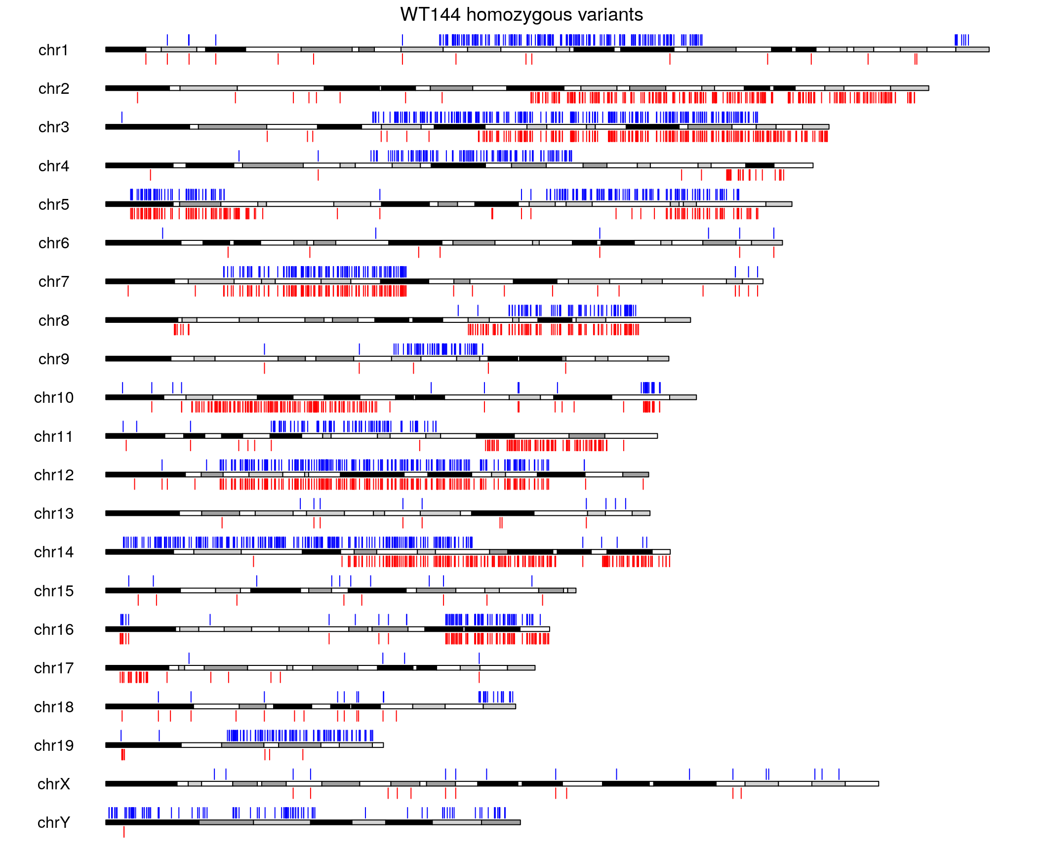
| Version | Author | Date |
|---|---|---|
| 7ee5a38 | xhyuo | 2023-03-15 |
#save plot
pdf(file = "output/WT144_variants_nointersect_noindels_homo.pdf", width = 11, height = 9)
pp <- getDefaultPlotParams(plot.type=2)
pp$data1height <- 140
pp$data2height <- 140
pp$topmargin <- 300
kp <- plotKaryotype(genome = "mm10", plot.type = 2, plot.params = pp)
kpAddMainTitle(kp, main="WT144 homozygous variants", cex = 1.2)
kpDataBackground(kp, data.panel = 1, color = "white")
kpDataBackground(kp, data.panel = 2, color = "white")
kpPlotRegions(kp, data=snp1, col="blue", avoid.overlapping = FALSE, r0 = 0, r1 = 0.8, data.panel = 1)
kpPlotRegions(kp, data=snp2, col="red",  avoid.overlapping = FALSE, r0 = 0, r1 = 0.8, data.panel = 2)
dev.off()
png
2 WT144 QTL interval
#genes in the qtl region
query_variants <- create_variant_query_func("/projects/compsci/vmp/USERS/heh/DO_Opioid/data/cc_variants.sqlite")
query_genes <- create_gene_query_func("/projects/compsci/vmp/USERS/heh/DO_Opioid/data/mouse_genes_mgi.sqlite")

#chr5 interval-----------------------------------------------------------------------
#the interval for chr5 is 72.40547 to 77.76853 cM, in bp is 133052642 to 138956439
#Ssc4d at chr5 135.9602 - 135.9745; MGI:MGI:1924709
chr5_gene <- query_genes(chr = 5, 129, 139) %>%
  dplyr::filter(!str_detect(Name, "^Gm")) # remove gene starting with Gm
  # dplyr::mutate(Name = case_when(
  #   str_detect(Name, "^Gm") ~ "",
  #   TRUE ~ as.character(Name)
  #   ))

#variant
vcf.file3 = "/projects/compsci/legacy/USERS/peera/Kumar_lab/WT144_markers/final_list_of_markers.vcf"
vcf3 = read.vcfR(vcf.file3)
Scanning file to determine attributes.
File attributes:
meta lines: 108
header_line: 109
variant count: 340
column count: 11
Meta line 108 read in.
All meta lines processed.
gt matrix initialized.
Character matrix gt created.
Character matrix gt rows: 340
Character matrix gt cols: 11
skip: 0
nrows: 340
row_num: 0
Processed variant: 340
All variants processed#snp
chr5.region <- vcf3@fix %>%
as.data.frame() %>%
dplyr::mutate(POS = as.numeric(POS)) %>%
dplyr::mutate(eff = str_match(INFO, ";EFF=\\s*(.*?)\\s*;")[,2]) %>%
dplyr::mutate(anno = gsub("\\(.*", "", eff)) %>%
dplyr::filter(CHROM == "chr5") %>%
dplyr::filter(between(POS, 129*1e6, 139*1e6))
chr5.region <- chr5.region %>%
dplyr::mutate(anno = factor(anno, levels = c("INTRON", "INTERGENIC", "DOWNSTREAM", "EXON", "NON_SYNONYMOUS_CODING")))
# 2 x 1 panels; adjust margins
old_mfrow <- par("mfrow")
old_mar <- par("mar")
on.exit(par(mfrow=old_mfrow, mar=old_mar))
layout(rbind(1,2), heights=c(2, 4))
top_mar <- bottom_mar <- old_mar
top_mar <- c(0.01, 10, 2, 2)
bottom_mar <- c(5.10, 10, 0.01, 2)
par(mar=top_mar)
#Create the base plot
plot(chr5.region$POS, chr5.region$anno, type = "n", xaxt = "n", xaxs = "i",
xlim = c(1.29e08, 1.40e08),
xlab = "",ylab = "", yaxt = "n", main = "WT144 Chr5 QTL interval")
#axis(1, at = seq(1.29e08, 1.40e08, by = 2e6), las=1, padj = -1) #make sure top and bottom x axis aligned
# Add points to the plot
points(chr5.region$POS, chr5.region$anno, pch = "|", cex = 1, col = "red")
box() # Add a box around the plot
# Change the y-axis tick labels
axis(2, 1:length(levels(chr5.region$anno)), labels = levels(chr5.region$anno), las = 1, cex.axis = 0.65)
#bottom
par(mar=bottom_mar)
plot_genes(chr5_gene, bgcolor="white",
xlim = c(1.29e08/1e6, 1.40e08/1e6))
axis(1, at = seq(1.29e08, 1.40e08, by = 2e6),
labels = seq(1.29e08, 1.40e08, by = 2e6)/1e6,
las=1, padj = -1)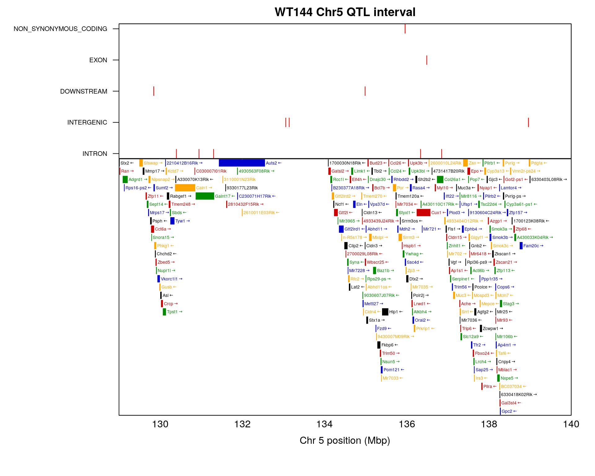
# save the plot
pdf(file = "output/wt144_chr5_qtlinterval.pdf", width = 10, height = 8)
old_mfrow <- par("mfrow")
old_mar <- par("mar")
on.exit(par(mfrow=old_mfrow, mar=old_mar))
layout(rbind(1,2), heights=c(2, 4))
top_mar <- bottom_mar <- old_mar
top_mar <- c(0.01, 10, 2, 2)
bottom_mar <- c(5.10, 10, 0.01, 2)

par(mar=top_mar)
#Create the base plot
plot(chr5.region$POS, chr5.region$anno, type = "n", xaxt = "n", xaxs = "i",
     xlim = c(1.29e08, 1.40e08),
     xlab = "",ylab = "", yaxt = "n", main = "WT144 Chr5 QTL interval")
#axis(1, at = seq(1.29e08, 1.40e08, by = 2e6), las=1, padj = -1) #make sure top and bottom x axis aligned
# Add points to the plot
points(chr5.region$POS, chr5.region$anno, pch = "|", cex = 1, col = "red")
box()  # Add a box around the plot
# Change the y-axis tick labels
axis(2, 1:length(levels(chr5.region$anno)), labels = levels(chr5.region$anno), las = 1, cex.axis = 0.65)
#bottom
par(mar=bottom_mar)
plot_genes(chr5_gene, bgcolor="white",
           xlim = c(1.29e08/1e6, 1.40e08/1e6))
axis(1, at = seq(1.29e08, 1.40e08, by = 2e6),
     labels = seq(1.29e08, 1.40e08, by = 2e6)/1e6,
     las=1, padj = -1)
dev.off()
png
2 #chr14 interval-----------------------------------------------------------------------
#the interval for chr14 is 26.14972 to 36.07219 cM, in bp is 50642778 to 69691477
#Kpna3 at chr14 61.36519 - 61.43995; MGI:MGI:1100863
chr14_gene <- query_genes(chr = 14, 59.642778, 69.691477) %>%
dplyr::filter(!str_detect(Name, "^Gm")) # remove gene starting with Gm
#snp
chr14.region <- vcf3@fix %>%
as.data.frame() %>%
dplyr::mutate(POS = as.numeric(POS)) %>%
dplyr::mutate(eff = str_match(INFO, ";EFF=\\s*(.*?)\\s*;")[,2]) %>%
dplyr::mutate(anno = gsub("\\(.*", "", eff)) %>%
dplyr::filter(CHROM == "chr14") %>%
dplyr::filter(between(POS, 59.642778*1e6, 69.691477*1e6)) %>%
dplyr::mutate(anno = as.factor(anno))
# 2 x 1 panels; adjust margins
# 2 x 1 panels; adjust margins
old_mfrow <- par("mfrow")
old_mar <- par("mar")
on.exit(par(mfrow=old_mfrow, mar=old_mar))
layout(rbind(1,2), heights=c(2, 4))
top_mar <- bottom_mar <- old_mar
top_mar <- c(0.01, 10, 2, 2)
bottom_mar <- c(5.10, 10, 0.01, 2)
par(mar=top_mar)
#Create the base plot
plot(chr14.region$POS, chr14.region$anno, type = "n", xaxt = "n", xaxs = "i",
xlim = c(61e06, 70e06),
xlab = "",ylab = "", yaxt = "n", main = "WT144 chr14 QTL interval")
#axis(1, at = seq(61e06, 70e06, by = 2e6), las=1, padj = -1) #make sure top and bottom x axis aligned
# Add points to the plot
points(chr14.region$POS, chr14.region$anno, pch = "|", cex = 1, col = "red")
box() # Add a box around the plot
# Change the y-axis tick labels
axis(2, 1:length(levels(chr14.region$anno)), labels = levels(chr14.region$anno), las = 1, cex.axis = 0.65)
#bottom
par(mar=bottom_mar)
plot_genes(chr14_gene, bgcolor="white",
xlim = c(61e06/1e6, 70e06/1e6))
axis(1, at = seq(61e06, 70e06, by = 2e6),
labels = seq(61e06, 70e06, by = 2e6)/1e6,
las=1, padj = -1)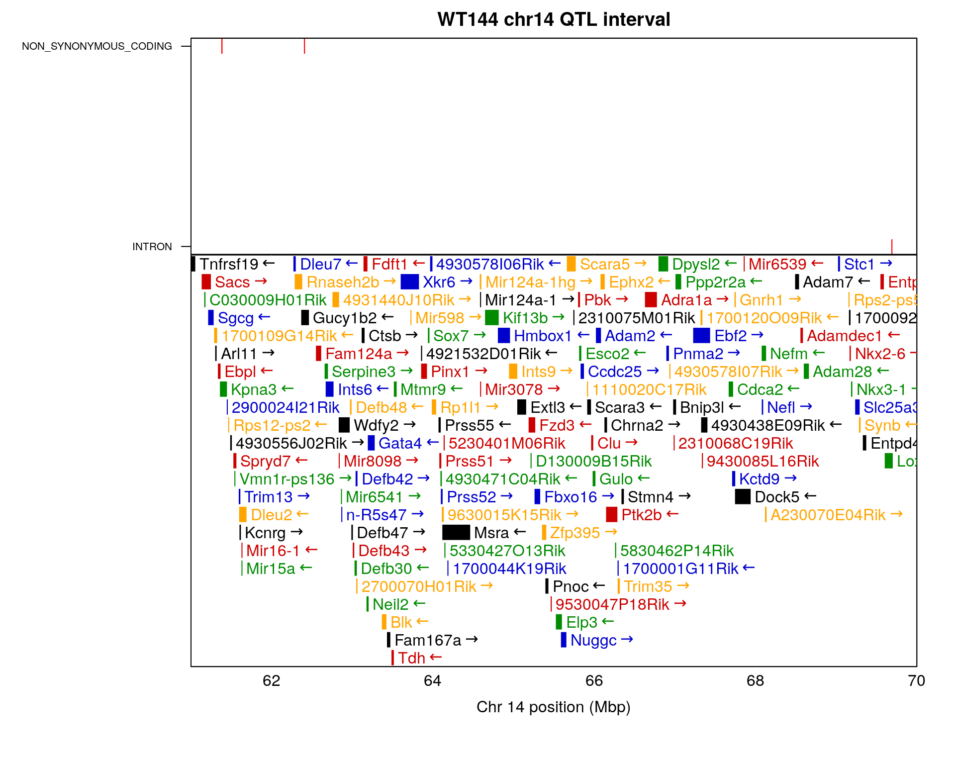
# save the plot
pdf(file = "output/wt144_chr14_qtlinterval.pdf", width = 10, height = 8)
# 2 x 1 panels; adjust margins
old_mfrow <- par("mfrow")
old_mar <- par("mar")
on.exit(par(mfrow=old_mfrow, mar=old_mar))
layout(rbind(1,2), heights=c(2, 4))
top_mar <- bottom_mar <- old_mar
top_mar <- c(0.01, 10, 2, 2)
bottom_mar <- c(5.10, 10, 0.01, 2)

par(mar=top_mar)
#Create the base plot
plot(chr14.region$POS, chr14.region$anno, type = "n", xaxt = "n", xaxs = "i",
     xlim = c(61e06, 70e06),
     xlab = "",ylab = "", yaxt = "n", main = "WT144 chr14 QTL interval")
#axis(1, at = seq(61e06, 70e06, by = 2e6), las=1, padj = -1) #make sure top and bottom x axis aligned
# Add points to the plot
points(chr14.region$POS, chr14.region$anno, pch = "|", cex = 1, col = "red")
box()  # Add a box around the plot
# Change the y-axis tick labels
axis(2, 1:length(levels(chr14.region$anno)), labels = levels(chr14.region$anno), las = 1, cex.axis = 0.65)
#bottom
par(mar=bottom_mar)
plot_genes(chr14_gene, bgcolor="white",
           xlim = c(61e06/1e6, 70e06/1e6))
axis(1, at = seq(61e06, 70e06, by = 2e6),
     labels = seq(61e06, 70e06, by = 2e6)/1e6,
     las=1, padj = -1)
dev.off()
png
2 #chr5 and chr14 in one figure-----------------------------------------------------
layout(mat = matrix(c(1:4),
nrow = 2,
ncol = 2),
heights = c(1, 2), # Heights of the two rows
widths = c(3, 2.25)) # Widths of the two columns
# Plot 1
par(mar = c(0.01, 10, 2, 0.5))
#Create the base plot
plot(chr5.region$POS, chr5.region$anno, type = "n", xaxt = "n", xaxs = "i",
xlim = c(1.29e08, 1.40e08),
xlab = "",ylab = "", yaxt = "n", main = "WT144 Chr5 QTL interval")
#axis(1, at = seq(1.29e08, 1.40e08, by = 2e6), las=1, padj = -1) #make sure top and bottom x axis aligned
# Add points to the plot
points(chr5.region$POS, chr5.region$anno, pch = "|", cex = 2, col = "red")
box() # Add a box around the plot
# Change the y-axis tick labels
axis(2, 1:length(levels(chr5.region$anno)), labels = levels(chr5.region$anno), font = 2, las = 1, cex.axis = 0.7)
# text(136332619, # Add labels
# 5,
# labels = "Chr5-136332619-.-C-A",
# pos = 4, offset = 0.1,
# cex = 0.5)
# Plot 2
par(mar = c(5.10, 10, 0.01, 0.5))
plot_genes(chr5_gene, bgcolor="white",
xlim = c(1.29e08/1e6, 1.40e08/1e6))
axis(1, at = seq(1.29e08, 1.40e08, by = 2e6),
labels = seq(1.29e08, 1.40e08, by = 2e6)/1e6,
las=1, padj = -1)
# Plot 3
par(mar = c(0.01, 0.01, 2, 0.5))
#Create the base plot
plot(chr14.region$POS, chr14.region$anno, type = "n", xaxt = "n", xaxs = "i",
xlim = c(61e06, 70e06),
xlab = "", ylab = "", yaxt = "n", main = "WT144 chr14 QTL interval")
#axis(1, at = seq(61e06, 70e06, by = 2e6), las=1, padj = -1) #make sure top and bottom x axis aligned
# Add points to the plot
points(chr14.region$POS, chr14.region$anno, pch = "|", cex = 2, col = "red")
box() # Add a box around the plot
# Change the y-axis tick labels
axis(2, 1:length(levels(chr14.region$anno)), labels = FALSE, las = 1, font = 2, cex.axis = 0.7, tick = FALSE)
# text(69691477, # Add labels
# 1,
# labels = "Chr14-69691477-.-G-T",
# pos = 2, offset = 0.1,
# cex = 0.5)
# Plot 4
par(mar = c(5.10, 0.01, 0.01, 0.5))
plot_genes(chr14_gene, bgcolor="white",
xlim = c(61e06/1e6, 70e06/1e6))
axis(1, at = seq(61e06, 70e06, by = 2e6),
labels = seq(61e06, 70e06, by = 2e6)/1e6,
las=1, padj = -1)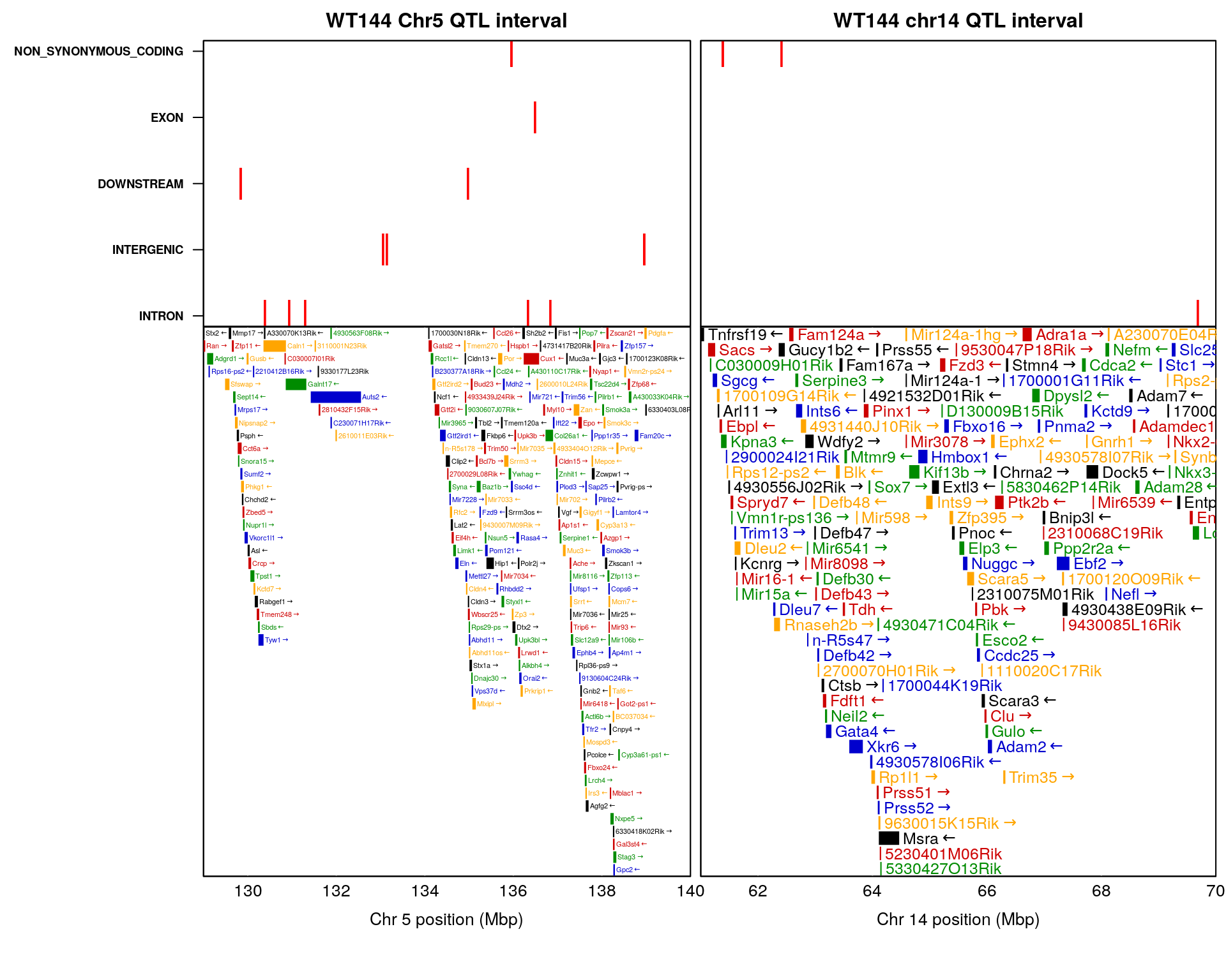
# save the plot
pdf(file = "output/wt144_chr5_and_chr14_qtlinterval.pdf", width = 11, height = 8.3)# Set plot layout
layout(mat = matrix(c(1:4),
                    nrow = 2,
                    ncol = 2),
       heights = c(1, 2),    # Heights of the two rows
       widths = c(3, 2.25))     # Widths of the two columns

# Plot 1
par(mar = c(0.01, 10, 2, 0.5))
#Create the base plot
plot(chr5.region$POS, chr5.region$anno, type = "n", xaxs = "i",
     xlim = c(1.29e08, 1.40e08),
     xlab = "",ylab = "", yaxt = "n", main = "WT144 Chr5 QTL interval")
#axis(1, at = seq(1.29e08, 1.40e08, by = 2e6), las=1, padj = -1) #make sure top and bottom x axis aligned
# Add points to the plot
points(chr5.region$POS, chr5.region$anno, pch = "|", cex = 2, col = "red")
box()  # Add a box around the plot
# Change the y-axis tick labels
axis(2, 1:length(levels(chr5.region$anno)), labels = levels(chr5.region$anno), font = 2, las = 1, cex.axis = 0.7)
# text(136332619,                                # Add labels
#      5,
#      labels = "Chr5-136332619-.-C-A",
#      pos = 4, offset = 0.1,
#      cex = 0.5)

# Plot 2
par(mar = c(5.10, 10, 0.01, 0.5))
plot_genes(chr5_gene, bgcolor="white",
           xlim = c(1.29e08/1e6, 1.40e08/1e6))
axis(1, at = seq(1.29e08, 1.40e08, by = 2e6),
     labels = seq(1.29e08, 1.40e08, by = 2e6)/1e6,
     las=1, padj = -1)

# Plot 3
par(mar = c(0.01, 0.01, 2, 0.5))
#Create the base plot
plot(chr14.region$POS, chr14.region$anno, type = "n", xaxt = "n", xaxs = "i",
     xlim = c(61e06, 70e06),
     xlab = "", ylab = "", yaxt = "n", main = "WT144 chr14 QTL interval")
#axis(1, at = seq(61e06, 70e06, by = 2e6), las=1, padj = -1) #make sure top and bottom x axis aligned
# Add points to the plot
points(chr14.region$POS, chr14.region$anno, pch = "|", cex = 2, col = "red")
box()  # Add a box around the plot
# Change the y-axis tick labels
axis(2, 1:length(levels(chr14.region$anno)), labels = FALSE, las = 1, font = 2, cex.axis = 0.7, tick = FALSE)
# text(69691477,                                # Add labels
#      1,
#      labels = "Chr14-69691477-.-G-T",
#      pos = 2, offset = 0.1,
#      cex = 0.5)

# Plot 4
par(mar = c(5.10, 0.01, 0.01, 0.5))
plot_genes(chr14_gene, bgcolor="white",
           xlim = c(61e06/1e6, 70e06/1e6))
axis(1, at = seq(61e06, 70e06, by = 2e6),
     labels = seq(61e06, 70e06, by = 2e6)/1e6,
     las=1, padj = -1)
dev.off()
png
2
sessionInfo()R version 4.0.3 (2020-10-10)
Platform: x86_64-pc-linux-gnu (64-bit)
Running under: Ubuntu 20.04.2 LTS
Matrix products: default
BLAS/LAPACK: /usr/lib/x86_64-linux-gnu/openblas-pthread/libopenblasp-r0.3.8.so
locale:
[1] LC_CTYPE=en_US.UTF-8 LC_NUMERIC=C
[3] LC_TIME=en_US.UTF-8 LC_COLLATE=en_US.UTF-8
[5] LC_MONETARY=en_US.UTF-8 LC_MESSAGES=C
[7] LC_PAPER=en_US.UTF-8 LC_NAME=C
[9] LC_ADDRESS=C LC_TELEPHONE=C
[11] LC_MEASUREMENT=en_US.UTF-8 LC_IDENTIFICATION=C
attached base packages:
[1] stats4 parallel stats graphics grDevices utils datasets
[8] methods base
other attached packages:
[1] qtl2_0.24 biomaRt_2.46.3
[3] vcfR_1.12.0 karyoploteR_1.16.0
[5] regioneR_1.22.0 ensemblVEP_1.32.1
[7] VariantAnnotation_1.36.0 SummarizedExperiment_1.20.0
[9] Biobase_2.50.0 MatrixGenerics_1.2.1
[11] matrixStats_0.58.0 data.table_1.13.6
[13] Rsamtools_2.6.0 Biostrings_2.58.0
[15] XVector_0.30.0 GenomicRanges_1.42.0
[17] GenomeInfoDb_1.26.7 IRanges_2.24.1
[19] S4Vectors_0.28.1 BiocGenerics_0.36.1
[21] forcats_0.5.1 stringr_1.4.0
[23] dplyr_1.0.4 purrr_0.3.4
[25] readr_1.4.0 tidyr_1.1.2
[27] tibble_3.0.6 ggplot2_3.3.3
[29] tidyverse_1.3.0 workflowr_1.6.2
loaded via a namespace (and not attached):
[1] readxl_1.3.1 backports_1.2.1 Hmisc_4.4-2
[4] BiocFileCache_1.14.0 lazyeval_0.2.2 splines_4.0.3
[7] BiocParallel_1.24.1 digest_0.6.27 ensembldb_2.14.1
[10] htmltools_0.5.1.1 magrittr_2.0.1 checkmate_2.0.0
[13] memoise_2.0.0 BSgenome_1.58.0 cluster_2.1.1
[16] modelr_0.1.8 askpass_1.1 prettyunits_1.1.1
[19] jpeg_0.1-8.1 colorspace_2.0-0 blob_1.2.1
[22] rvest_0.3.6 rappdirs_0.3.3 haven_2.3.1
[25] xfun_0.21 crayon_1.4.1 RCurl_1.98-1.2
[28] jsonlite_1.7.2 ape_5.4-1 survival_3.2-7
[31] glue_1.4.2 gtable_0.3.0 zlibbioc_1.36.0
[34] DelayedArray_0.16.3 scales_1.1.1 bezier_1.1.2
[37] DBI_1.1.1 Rcpp_1.0.6 viridisLite_0.3.0
[40] progress_1.2.2 htmlTable_2.1.0 foreign_0.8-81
[43] bit_4.0.4 Formula_1.2-4 htmlwidgets_1.5.3
[46] httr_1.4.2 RColorBrewer_1.1-2 ellipsis_0.3.1
[49] pkgconfig_2.0.3 XML_3.99-0.5 nnet_7.3-15
[52] dbplyr_2.1.0 tidyselect_1.1.0 rlang_1.0.2
[55] later_1.1.0.1 AnnotationDbi_1.52.0 munsell_0.5.0
[58] cellranger_1.1.0 tools_4.0.3 cachem_1.0.4
[61] cli_2.3.0 generics_0.1.0 RSQLite_2.2.3
[64] broom_0.7.4 evaluate_0.14 fastmap_1.1.0
[67] yaml_2.2.1 knitr_1.31 bit64_4.0.5
[70] fs_1.5.0 AnnotationFilter_1.14.0 nlme_3.1-152
[73] whisker_0.4 xml2_1.3.2 compiler_4.0.3
[76] rstudioapi_0.13 curl_4.3 png_0.1-7
[79] reprex_1.0.0 stringi_1.5.3 highr_0.8
[82] GenomicFeatures_1.42.3 memuse_4.1-0 lattice_0.20-41
[85] ProtGenerics_1.22.0 Matrix_1.3-2 permute_0.9-5
[88] vegan_2.5-7 vctrs_0.3.6 pillar_1.4.7
[91] lifecycle_1.0.0 bitops_1.0-6 httpuv_1.5.5
[94] rtracklayer_1.50.0 R6_2.5.0 latticeExtra_0.6-29
[97] promises_1.2.0.1 gridExtra_2.3 dichromat_2.0-0
[100] MASS_7.3-53.1 assertthat_0.2.1 openssl_1.4.3
[103] rprojroot_2.0.2 pinfsc50_1.2.0 withr_2.4.1
[106] GenomicAlignments_1.26.0 GenomeInfoDbData_1.2.4 mgcv_1.8-34
[109] hms_1.0.0 grid_4.0.3 rpart_4.1-15
[112] bamsignals_1.22.0 rmarkdown_2.6 git2r_0.28.0
[115] biovizBase_1.38.0 lubridate_1.7.9.2 base64enc_0.1-3